This document is for the NodeBrain rule engine, an open source agent for state and event monitoring applications. The NodeBrain language syntax and symantics are fully described in this document. Readers new to NodeBrain are encouraged to start with the NodeBrain Tutorial, which introduces concepts using simple examples. Reference NodeBrain Guide for general information about using the rule engine and related components.
Release 0.9.03, December 2014
Copyright © 2014 Ed Trettevik <eat@nodebrain.org>
Permission is granted to copy, distribute and/or modify this document under the terms of either the MIT License (Expat) or NodeBrain License. See the Licenses section at the end of this document for details.
Short Table of Contents
This chapter introduces some basic concepts of the NodeBrain language. It is intended as an overview to provide a foundation for understanding, not as a rigorous and complete description. Most of these topics will be covered in more detail in later chapters.
A string is stored internally as a null terminated sequence of characters. You represent a string by enclosing a sequence of character in quotes.
     	"abc"
     	"This is a string."
There are no string manipulation operators in NodeBrain, although symbolic substitution is supported and enables symbolic command construction. String comparisons and regular expression matching is supported.
     	A<"george"	[String comparison]
     	A~"^abc.*d+$"	[Regular expression match]
Modules provide cell functions for additional operations on strings.
Numbers are stored internally as floating-point values. You represent numbers with a sequence of decimal digits with an optional plus or minus sign, decimal point, and exponent.
            127
            -3.23456e+10
            4.5
            +7
Only the basic operations of addition, subtraction, multiplication, and division are supported by operators. Modules provide cell functions for additional numerical operations.
Special symbols are used to represent the logical values of True, False and Unknown. Also, the logical value of True can be represented by any number or string.
| Value | Logical
|
|---|---|
| ? | unknown
|
| ! | false
|
| !! | true
|
| 1 | true
|
| 0 | true
|
| "abc" | true
|
| 27 | true
|
| -5.4 | true
|
This deviates from the common practice of using zero to represent false, with the goal of
enabling operators to discriminate against False without discriminating against 0.
For example, the formula A false "abc" evaluates to the value of A unless it is False, in which
case it evaluates to "abc". If False were represented by 0, this formula could never return 0,
and any formula that could return 0 could not avoid having its value interpreted as false.
A formula is a simple value (e.g. number, string, True, False, and Unknown), or an expression that computes a value. For a simple numerical calcuation, a formula may include the operators for addition (+), subtraction (-), multiplication (*), and division (/).
             5*2+10
             21/3-2
A formula may also include relational and logical operators.
| Logical Expression
|
|---|
| a>17
|
| a>5 and b<2
|
| a and !b and c="abc"
|
An extensive set of time related operators are included, with a chapter devoted to the topic. The expression below is true from 2:00 AM to 3:00 AM on Tuesday of the week of the last Friday in January and June.
| Logical Expression
|
|---|
| ~(h(2).tu.w.fr[-1](jan,jun))
|
The interpreter enables bindings to external function libraries, making the external functions available as cell functions. Several cell functions are provided for common math functions. Examples of cell function calls are shown in the table below.
| Cell Function Call | Result
|
|---|---|
| `math.mod(45,2) | 1
|
| `math.floor(16.2345) | 16
|
| `math.exp(35.5) | e^35.4
|
NodeBrain also supports node function calls that look like normal function calls, but act a bit like class methods in an object oriented language because they operate on an instance of a type of information, where the type determines the functions available. The logic for these functions is provided by external modules while the interpreter manages the scheduling of the calls to these functions.
| Node Function Call
|
|---|
| WatchedMachineUser(a,b)
|
| MyTable@rows(a,b,c)
|
A cell is a container of both a value and a formula from which the value is computed. For simple cells, the formula and value are identical.
| Cell Formula | Cell Value
|
|---|---|
| "abc" | "abc"
|
| 0 | 0
|
| ? | ?
|
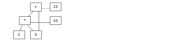
For more complex cells, the formula includes references to operators that derive values from the value of other cells (operands). This concept is illustrated below with multiplication (*) and addition (+) operators.
| Cell Formula | Cell Value
|
|---|---|
| 5*2 | 10
|
| 10+5 | 15
|
A formula is a unique identifier of a cell. In other words, only one cell exists for a given formula. Any number of cells may reference a given cell. In the example above, the two complex cells, (5*2) and (10+5), reference three simple cells (2, 5, and 10). A complex cell may reference other complex cells. For example, the definition below creates a cell that references the existing simple cell 5 and the existing complex cell (5*2).
| Cell Formula | Cell Value
|
|---|---|
| 5*2+5 | 15
|
A cell formula may be much more complicated, as illustrate in the previous section. Formulas often include terms that can act like variables or functions.
In general, a term is an identifier used to represent knowledge. For now, let's look at the most common case, where a term is used as a cell. These terms reference cells and are themselves cells. In the set of examples below, you assert values for the terms A through E and "fred" by the cell expressions following the equal symbol (=) or double equal symbol (==). A single equal references the value of the cell expression at the time of the assertion. A double equal references the value of the cell expression from the time of the assertion and into the future. In this example, the value of E will automatically change if A or D changes.
assert A=3,B="abc",C=1.5,D=3*5,E==A*D,fred=`math.mod(E,17)+25.67;
It is best to think of a term as an alias. It is a cell that simply references another cell. A term, like all cells, can be referenced by other cells. The value of a term is the value of the cell it currently references. So A=3, D=15, and E=45 based on the definitions above.
You can change the value of a term by changing the cell it references. Below, you change the values of A and D to the values of 4 and 3*7 respectively by changing their formulas to new constants.
assert A=4,D=3*7;
The new values are A=4, D=21, and E=84. Notice the value of E changed automatically as a result of the change to A and D. This is an important concept in NodeBrain. When you assert that E==A*D, you didn't just assign E the current value of A*D (45), you also defined a formula for computing E. It is the same formula as that used by the cell "named" A*D, for which E is currently an alias.
A condition is a cell for which the value is reduced to True, False, or Unknown. All values other than False (!) and Unknown (?) map to True when interpreted as a condition.
This means any cell may be used as a condition or an operand within a condition.
Some operators are designed specifically for use in conditions. Examples include relational operators (=, >, >=, <, <=, and <>) and trinary logic operators (&, |, and !). The words "and" and "or" may be used as alternatives to & and | respectively.
     a>1            [a greater than 1]
     b<>a           [b not equal to a]
     a & !b         [a and !b]
     a and !b       [a & !b]
Trinary logic operators allow for an Unknown value, extending Boolean logic, which has only True and False values.
The following table shows this extension for the logical and (&) operator.
The symbol !! is a special case of True that is returned by some logical operators.
| A | B | A & B
|
|---|---|---|
| ! | ! | !
|
| ! | !! | !
|
| ! | ? | !
|
| !! | ! | !
|
| !! | !! | !!
|
| !! | ? | ?
|
| ? | ! | !
|
| ? | !! | ?
|
| ? | ? | ?
|
Relational operators like >, <, and = always return Unknown when one of their operands is Unknown, and when a number is compared to a string.
Now let's look at an example.
     assert X==(A>B & C=5);
     assert A=7;
     assert C=4;
If this is all the information you have, then B is Unknown; that is, B=?. However, the value of B is not needed to determine that X=! because (C=5) is ! and (? & !) is !.
In procedural languages, conditional expressions are evaluated when the statement containing the expression is executed. In NodeBrain, individual cells are evaluated when the value of any referenced cell changes. (This is similar to cells in a spreadsheet.) The following assertion will not cause evaluation of X because the value of A does not change—it is still 7 after the assertion.
assert A==C+3;
If you then make the following assertion, A becomes 8 (5+3) and X becomes True (!!). To clarify, X is the result of (8>1 & 5=5) or (!! & !!), which is !!.
assert C=5,B=1;
In addition to the common operators used within conditions, NodeBrain has special operators with memory and time awareness.
     A ^ B                  [flip-flop]
     team(A,B,C)            [node sentence formula]
     ~(h(4).su[3]jan)       [time condition]
     A ~^(10m)              [time delay]
We won't go into the details of these operators here, but they are important features of the language to cover later.
Rules are used to define the conditions you want NodeBrain to monitor and the desired actions or responses to specific conditions. There are three types of rules: on, when, and if. Other than the type identifier, the syntax is the same.
     define term on(condition) assertion: command
     define term when(condition) assertion: command
     define term if(condition) assertion: command
An on rule will fire any time the condition transitions to a True value from a non-True value (False or Unknown). When a rule fires, the action may include an assertion and a NodeBrain command. If a condition is True at the time a rule is defined, this does not qualify as a transition to a True state. In that case, the condition must first transition to False or Unknown and then transition to True.
A when rule behaves just like an on rule, except it only fires once. After a when rule fires, it is removed from the interpreter's memory.
The syntax for the optional assertion clause is just like the syntax illustrated for the assert command, that is, a set of assignments separated by commas. This clause is interpreted with the define statement. An optional command follows the colon (:). This command is not interpreted until the rule fires and is re-interpreted each time the rule fires.
     define r1 on(a=1 and b=2) c="xyz",x=25;
     define r2 on(c="xyz"): command2
     define r3 when(x>20) e=5.246: command3
     define r4 if(a=1 and b=2): command4
     define r5 if(a>17); # This rule has no action
The value of rule conditions changes in response to assert and alert commands and the system clock for time conditions. Except for the verb, the assert and alert commands have identical syntax as illustrated by the following examples.
     assert a=1,b=2;
     alert a=1,b=2;
For on and when rules, no distinction is made between assert and alert. For the purpose of condition value update, this is also true of if rules. However, the firing mechanism is different for if rules. An if rule will only fire on an alert command and it will always fire when True. It does not require a transition from another state.
You may think of an alert command as a representation of an "event" and the if rule as an "event monitoring" rule. You may also think of an assert command as a representation of a "state," and the on rule as a "state monitoring" rule. However, remember that conditions for all rules respond to both assert and alert in a consistent way. This means if rules may be used for "stateful event monitoring," where conditions are based on asserted states as well as event attributes provided by alerts.
The when rule shows no preference toward either of the concepts of "state" or "event." A when rule may be defined to watch for a specific "state" or "event," take some action, and disappear.
A set of rules may be written to implement a state transition table.
     define r1r on(state=1 and red) state=2: actionA
     define r1g on(state=1 and green) state=3: actionB
     define r1b on(state=1 and blue) state=4;
     define r2g on(state=2 and green) state=3;
     define r3r on(state=3 and red) ?state: actionC
     define r4y on(state=4 and yellow) state=5: actionD
     define r5r on(state=5 and red) ?state;
     define r5g on(state=5 and green) state=1;
A node is an object with special knowledge and the skill to use it within the framework provided by NodeBrain.
In the simplest form, a node is a set of rules and supporting terms that work together to monitor the state of one or more elements,
or monitor an event stream. Terms are defined within the context of a node. Examples in previous sections have defined all terms at the
top level node. Here's an example were terms are defined within a subordinate node called my.
     define my node;
     my. define x cell;
     my. define y cell;
     my. define r1 on(x>y):alert type="InvertedConflugification";
     define tellMy on(a=b) my.x=2,my.y=1;
Additional capabilities for a node are often provided by a node module, and additinal knowledge is either asserted using NodeBrain commands or obtained from an external source.
A node module implements a type of node by providing functions (methods) that NodeBrain calls to handle specific tasks like assertion, evaluation, and command interpretation. For example, suppose you have a node module named myskill. You could define a node named shania and reference it as shown below.
     define shania node myskill;
     define r1 on(shania("abc",20)) a=7;
     assert shania(1,3,5)=30,shania(5,"ready");
     shania:This is a message handled by myskill
     shania(1,"xyz"):This is another message with arguments
To understand the evaluation of shania("abc",20) and the assertions shania(1,3,5)=30 and shania(5,"ready") requires familiarity with the node module named myskill used to implement shania. NodeBrain simply asks the node module to handle the assertions and evaluations. When the value the node module returns for shania("abc",20) transitions to true, rule r1 fires and NodeBrain takes the action of asserting a=7.
To send a command (message) to a node, you begin a command with the node name followed by an optional argument list, followed by a colon (:). If a node module implements the command method, the argument list and text following the colon (:) are sent to the skill's command method. The interpretation of node commands is entirely up to the node module.
Manuals for modules distributed with NodeBrain are available at http://nodebrain.org. See the NodeBrain Library manual for information needed to write your own node modules.
A module is a plug-in to NodeBrain, normally implemented as a dynamically loaded shared library. These components extend NodeBrain by providing additional cell functions and/or node functions using the NodeBrain C API. This topic is covered in the NodeBrain Library manual. The model of interaction between modules and the interpreter relies heavily on modules registering callback functions when they are first loaded. This enables the rule engine (interpreter) to control the timing of calls based on events and state.
The NodeBrain language is a declarative language. With the exception of the %if source file directive and sequence rules, it does not have procedural flow of control constructs like IF-THEN-ELSE, CASE, WHILE, UNTIL, and FOR. It does not have sequential compound statements like "DO; ... END;" or "{...}". It does not support conventional user-defined functions or subroutines. It is not a general purpose programming language like C or Perl. NodeBrain is a special purpose declarative language. A NodeBrain programmer specifies rules that are similar to IF-THEN statements. However, the if conditions in NodeBrain, unlike those in procedural languages, are "constantly" being evaluated. There is no concept of "order" to the evaluation of rules.
On the other hand, commands are "executed" in the order they are presented to the interpreter. It may be helpful to think of a NodeBrain interpreter as a transaction processor. Each statement is a transaction that does one or more of the following:
If you think of a NodeBrain interpreter as a transaction processor, you can think of the set of data elements known to the interpreter as a primitive database. If you think of the data elements as simple "factual" knowledge and the cells and rules as more complex knowledge, you can think of the interpreter as a knowledge base. To a large extent, however, the interpreter's memory is volatile. When a NodeBrain process terminates, everything it "learned" (has been told) is forgotten. This can be overcome, to some extent, by writing rules that record information to *.nb files and load them at startup time. (But we're getting ahead of ourselves here.)
There are several ways to get commands to the interpreter: standard input file, queue files, TCP/IP socket connections, source files, shell command output, and translation of log files or other files with a syntax foreign to NodeBrain. In each of these cases, the commands are processed sequentially as presented to the interpreter.
In the previous section, you saw how commands are presented to the interpreter by itself when rules fire. In this case, you can make no assumptions about the sequence in which commands will be presented to the interpreter as rules fire. But there is some structure to the process described in the next section.
Now you will see more closely how NodeBrain reacts to assertions. As described earlier, assertions are made with assert and alert commands. You'll use assert commands and on rules in the examples here.
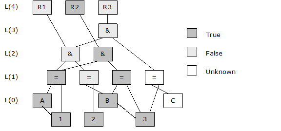
Suppose you have a brain with the following definitions.
     define R1 on(A=1 and B=2);
     define R2 on(A=1 and B=3);
     define R3 on(C=3 and A=1 and B=2);
If you display the conditions your brain is monitoring, it looks like the following. Seven cells are monitoring conditions. The value of each of these cells is unknown because the values of the terms a, b, and c are unknown.
     1  R[2]L(1) = ? == (A=1)
     2  R[1]L(1) = ? == (B=2)
     3  R[2]L(2) = ? == ((A=1)&(B=2))
     4  R[1]L(1) = ? == (B=3)
     5  R[1]L(2) = ? == ((A=1)&(B=3))
     6  R[1]L(1) = ? == (C=3)
     7  R[1]L(3) = ? == ((C=3)&((A=1)&(B=2)))
The R[2] on the first line tells you there are two references to the cell (A=1). This is interesting because you referenced (A=1) three times in the rules. The explanation is that rule R3 did not create a new reference to (A=1); it created a second reference to ((A=1)&(B=2)), which itself holds one of two references to (A=1). The other reference is held by ((A=1)&(B=3)).
The L(1) on the first line tells you (A=1) is a level 1 cell. Notice the second line shows a level 2 cell ((A=1)&(B=3)). This is an and cell referencing two level 1 cells: (A=1) and (B=3). Let's look at it graphically. Now the levels and references make sense.
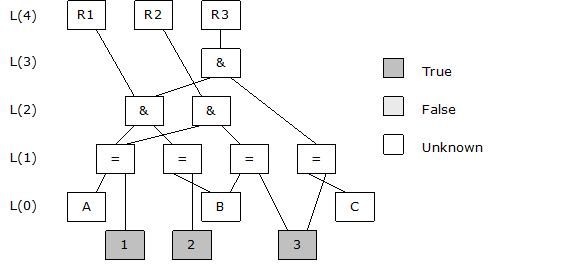
Within the internals of the NodeBrain interpreter you say that cell (A=1) has "subscribed" to changes in the value A, and that the cell ((A=1)&(B=2)) has subscribed to changes in the value of (A=1) and to the value of (B=2). Let's look at what happens when you make an assertion about A and B.
assert A=2,B=3;
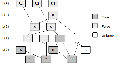
The impact of the changes to A and B are realized level by level. When A is assigned 2, this is a change, so A publishes a change to the (A=1) cell. This simply means (A=1) is scheduled for evaluation. When B is assigned 3, this is also a change, so B publishes a change to (B=2) and (B=3) because both have subscribed to changes in B.
After completing the assignments of the assert command, the interpreter enters an evaluation phase starting at level 1. There is no importance to the order in which (A=1), (B=2) and (B=3) are evaluated. Let's pretend they are evaluated in the order just listed. When (A=1) is evaluated, you discover it is False. This is a change, so both ((A=1)&(B=2)) and ((A=1)&(B=3)) are scheduled for evaluation. When (B=2) is evaluated, it too is False and the change is published to ((A=1)&(B=2)), which is already scheduled for evaluation. When (B=3) is evaluated, it is found to be True and the change is published to ((A=1)&(B=3)), which is also already scheduled for evaluation.
After completing level 1 evaluations, the interpreter repeats the process at level 2 and then level 3. All level 2 and level 3 cells are found to be False, so no rules fire.
Notice that condition (C=3) is still unknown but not necessary to determine that ((C=3)&((A=1)&(B=2))) is False.
Now suppose you make the following assertion.
assert a=1;
When A is assigned the value of 1, the interpreter schedules (A=1) for evaluation. If you were to trace the evaluation process, it might look like this.
     L(1): (A=1), True, This is a change so schedule subscribers for evaluation
     L(2): ((A=1)&(B=2)), (True & False), False, no change
     L(2): ((A=1)&(B=3)), (True & True), True, schedule R2 to fire
Notice it was not necessary to evaluate any condition directly referencing B or C because they did not change. Furthermore, it was not necessary to evaluate ((C=1)&((A=1)&(B=2))) because the value of the sub-expressions (C=1) and ((A=1)&(B=2)) never changed. The questions the interpreter had to answer were:
If you next assert that B=2, rule R1 will fire because (B=2) will be True, making ((A=1)&(B=2)) True. Rule R2 will reset because (B=3) will be False, making ((A=1)&(B=3)) False.
An assertion that C=3 will cause R3 to fire because ((A=1)&(B=2)) is already True.
An assertion that B=3 will cause R2 to fire again, and both R1 and R3 to reset.
There are two ways to begin a command cycle:
Once a command cycle begins, everything that happens until the interpreter is ready to accept another input command occurs within one command cycle.
Just as cells are scheduled for evaluation as described in the previous section, rules are scheduled to fire when their conditions are satisfied. Once NodeBrain schedules a rule to fire, it is committed to it. It simply starts stepping through the list of rules that are scheduled to fire and performs the specified actions. These actions may schedule new cell evaluations. It is quite possible that the actions of one rule will schedule cell evaluations that, if performed immediately, would change the state of other rule conditions before they actually fired. However, NodeBrain's cell evaluation algorithm doesn't care; it simply performs the actions of all scheduled rules. Then, if new cell evaluations have been scheduled, it starts a new "evaluation cycle," starting at level 1 and working up to the rule level. At the end of an evaluation cycle, if no new cell evaluations have been scheduled, the command cycle is complete.
Now consider the following rule set.
     define R1 on(!A) A;
     define R2 on(A) !A;
A command cycle, as described above, would be infinite if you asserted that !A with this rule set. To avoid this possibility, NodeBrain enforces an arbitrary limitation. No rule is allowed to fire more than once in a given command cycle. Under this limitation, a !A assertion will cause R1 to fire, which will assert A, causing R2 to fire, which will assert !A and the command cycle will end.
You can still have conflicts. Consider these rules.
     define R1 on(A=1) B=2;
     define R2 on(A=1) B=3;
What is the value of B after an assertion that A=1? All you can say is that the rule that fires last wins and, in general, you can't predict the order the rules will fire. You are advised not to create rules like this if you can help it. Currently NodeBrain does not prevent or identify this condition. It is fine and even desirable to allow a given term to change values more than once in a command cycle, so NodeBrain doesn't place a limitation on this like it did on rules firing more than once. But a future version may include logic that prevents (or at least detects) terms changing values multiple times in a single evaluation cycle's action phase.
A sequence rule in NodeBrain is a procedural construct expressed within a single command line enclosed in braces, "{...}". This feature is in an experimental state, so you should not rely on it for a production application. But it is worth an introduction, since the concept will be further developed in the future.
{=8;on(a=2);=5;10m;if(b=7)`c=3; }
The example above reads like this:
A sequence rule may be used as a command or a cell expression.
     > {on(a=1 and b=2)`c=7,b=4;on(a=2 and b=3)`c=2; }  # command
     > assert x=={=8;on(a=2);=5;10m;=9; }+b;            # cell expression
You can think of sequence rules (like all NodeBrain rules) as running concurrently under separate threads. These are called "correlation threads" because the primary purpose is to correlate a sequence of events.
The previous section showed how simple on rules can be used to implement a state table using a state variable. With sequence rules, a statement pointer provides a built-in state variable. The rule below responds to a sequence of green, blue, and red conditions.
{on(green);on(blue);on(red);action;}
Sequence rules are covered in more detail in Chapter 6, Rules.
Identifiers are used to reference objects ("things") by name, a concept you are familiar with from other programming languages. When the interpreter encounters a term identifier, it searches a hierarchical dictionary of terms to locate the referenced object. For a complete identifier, the search begins at the top of the dictionary. For a contextual identifier, the search is performed starting at a context term, often defined by a command context. A context term is aways a node.
Syntax
|
Constant numbers and strings also have unique identifiers that are distinct from terms. Furthermore, a formula is a unique identifier of a cell.
A term has a name, value, and definition. The name is the identifier, sometimes called a "term identifier" and more often just called a "term" when it is clear the name component is being discussed. A simple term is an alphanumeric string starting with an alpha character or an underscore. An underscore is not considered to be an alpha character, so may not be used after the first character of a term. The following are valid terms.
     APPLE
     Orange
     _blue
     reallySad
     happyCamper
     hikerBikerSurfer2
     three4five
When you use a term like a common variable, you assign a value using an assert command with a single equal symbol.
assert orange="You glad we didn't say banana?";
You can also use a term like a function by assigning a definition. This requires a double equal symbol.
assert Thomas==(ToB or !Tob);
That is the question, now what is the answer? It is explained later that Thomas is true when ToB is true or Tob is false, and otherwise Thomas is false or unknown. You really don't want to get into a painful discussion about logical expressions here. The point is simply that a term has simultaneously a definition and a value, both of which are NodeBrain objects. The definition of a term associated with cell is a formula.
Terms starting with an underscore "_" are reserved terms the interpreter or a module create for special reasons. You may reference these terms, but you don't get to invent them. (Just wanted to underscore the terms for using underscore terms.)
When you want to use a term that violates the syntax of a simple term, you may use a quoted term. This enables the use of recognizable names from foreign contexts as terms within NodeBrain rules. Any typable character, except a single quote (apostrophe, '), may be used between single quotes. (NodeBrain does not have an escape sequence for special characters.) The following are valid quoted terms.
     '/var/opt/goofy'
     'http://www.nodebrain.org'
It is important not to confuse a quoted term with a string. A quoted term is the name of something. A string is the name of itself. The following example asserts a string value for a quoted term.
assert 'http://www.nodebrain.org'="http://nodebrain.sourceforge.net";
A glossary is a set of terms. Every term may have a glossary of subordinate terms.
You reference a subordinate term by following a term with a period or an underscore and the subordinate term.
For example, x.A and x_A both reference a term A subordinate to a term x.
If x is, or is intended to be, a node, use x.A.
If x is not, or is intended not to be, a node, use x_A.
     term.subordinateTerm   [term is implied to be a node]
     term_subordinateTerm   [term is implied to not be a node]
This provides a way to organize information. For example, you might assert some information about employees within an employee node.
     assert employee.'Jane Dough'_salary=200000;
     assert employee.'Jane Dough'_title="Software Engineer";
     assert employee.'Jane Dough'_skill_programming_language_perl="expert";
     assert employee.'John Fawn'_salary=80000;
     assert employee.'John Fawn'_title="Software Apprentice Toady";
     assert employee.'John Fawn'_skill_programming_language_perl="novice";
Oops, bad example. Let's not monitor employees. Well, the concept also applies to things you do want to monitor. Just replace "employee" with "computer", "application", "process" or something else and then define the appropriate subordinate terms.
The use of underscore within terms was discontinued in release 0.6.4, and the use as separators within a multiple level qualified term was introduced in release 0.9.03. Prior to release 0.9.03, a period was used as the only separator and nodes had to be explicitly defined, otherwise they were assumed not to be nodes.
The use of "." as a separator following a node term, and "_" following non-node terms, enables the interpreter to
understand your intentions prior to a node being explicitly defined. Nodes are implicitly defined when a previously
undefined term is referenced as a node, either by the use of "." following the term or a refence to the term within a function call.
A function call reference is indicated by
a following @ or ( in the context of a formula, assertion or command verb, or a : in the context of a command verb.
If a node is explicitly defined after an implicit definition, there is no requirement to change the relationship
of if rules relative to nodes, since the implicit definition will have already established the intended relationship.
This is an important for the proper functioning of alert commands and if rules.
The define command may be used to redefine a term that was created implicitly.
The redefine command is required to redefine a term that was previously explicitly defined and not undefined.
It is important to remember that an identifier like 'John Fawn'_skill_programming_language_perl is not a single term.
Instead, it identifies a path to a term perl, perhaps one of many within the glossary structure (dictionary).
The followin undefine command will remove the last three lines in the example above.
All the subordinate terms of 'John Fawn' (salary, title, and skill)
and their subordinate terms are removed.
undefine employee.'John Fawn'
A dictionary is a complete hierarchy of terms and glossaries. Separate dictionaries are used for rules, calendars, modules, skills, symbolic terms, and so on.
This simply means there are multiple name spaces. Most terms are defined in the rule dictionary, explicitly with the define command or implicitly by referencing an undefined term.
     define A cell X+Y/Z;  # A is defined explicitly, whil X, Y, and Z are define implicitly
     assert B==X*Y;	      # B is defined explicitly, but implicitly with respect the "define" command
     foo. assert C=2;      # C is defined implicitly within an implicitly defined node named "foo"
Terms in dictionaries other than the rule dictionary are defined implicitly in some cases
and explicitly in others. However, the define command is only used for the rule dictionary.
Other dictionaries use the declare or %define command for explicit definitions.
Other dictionaries also do not use the "_" separator as described in the previous section.
They only use "." as the term separator
declare lunar module ./nb_moon.so;
When the interpreter needs to look up a term, the dictionary is understood by the syntax.
     assert x=a+b;             # x, a, and b are all looked up in the rule dictionary
     define moony node lunar;  # lunar is looked up in the skill or module dictionary
A context is a concept associated with nodes and the rule dictionary. Commands are interpreted within a given context. NodeBrain searches for terms up or down the glossary hierarchy starting from the glossary of a given node. You create a new context whenever you define a node.
define pie node;
You use a context prefix to tell the interpreter which node to use when interpreting a command. A context prefix is an identifier with a trailing period followed by a blank.
     identifier. verb body - statement with a context prefix
     verb body             - statement without a context prefix
Here you see two statements that would produce the same results, the second with a context prefix ("pie. "). Notice the difference to the right of the verb assert.
     assert pie.apple=5,pie.cherry=2,pie.pumpkin=8;
     pie. assert .apple=5,.cherry=2,.pumpkin=8;
Defining nodes within a node creates a context hierarchy.
In the example, the example below, the first line could be removed and the third line would implicitly define fresh as a node
because it is first referenced as a node in the context prefix.
     pie. define fresh node;
     pie. define dayold node;
     pie.fresh. assert .apple=1;  # pie.apple=5; pie.fresh.apple=1;
Prefixing the first term of a context identifier with periods directs the interpreter to a specific context relative to the current context.
     .identifier         - search the current context glossary
     ..identifier        - search the parent context glossary
     ...identifier   - search the grandparent context glossary
     ....identifier  - etc.
When searching for a context identifier that is not period-prefixed, the interpreter searches up the context hierarchy for the first term of the identifier, starting in the current context. This search may be resolved on any number of levels up the context hierarchy. The interpreter then resolves the remaining terms of the identifier by stepping down the glossary hierarchy one term at a time.
pie.apple - find "pie" in current or above, and find "apple" in "pie"
You can see an unconstrained upward search by modifying the earlier example. These modified commands are not equivalent in the specified order if "apple", "cherry", and "pumpkin" are not already defined in "pie", but are defined at a higher level. In that case, the first command would reference the higher level terms.
     pie. assert apple=5,cherry=2,pumpkin=8;
     assert pie.apple=5,pie.cherry=2,pie.pumpkin=8;
The underscore "_" symbol is used to reference the top level (root) context.
     _. assert x=1,y=2;
     assert _.x=1,_.y=2;
The context symbols, % and $, are used for contexts that contain special built-in terms or terms that apply only to the scope of the current source file or macro expansion. These are topics for other sections.
There are two primary constant data types, string and number. Constants have identifiers unique to the data type.
Syntax
|
A string identifier is, no surprise here, a sequence of characters enclosed in quotes. There is no escape symbol, so there is no way to include a quote in a string object.
     "process has failed"
     "threshold of 5 reached"
     "http://sourceforge.net"
Numbers are always stored as floating-point objects. The following numeric identifiers all reference the same number.
2100 2.1e+3 21.0e2
A number must always start with a numeric digit (0-9) or a sign (+ or -). Here are some more examples.
     0.45 - notice the leading zero used to start with a digit
     -3
     -4.567e-4
     -5e+21
     +52
When the interpreter encounters a constant, it is converted to an internal form, assigned a hash code, and looked up in a hash table specific to the data type. Since glossaries are also hash tables, and terms are assigned the same hash code as their name (term ABC and string "ABC" have a common hash code) one can think of constants as residing in a dictionary with only one level.
In the example below, you see the string constant "abc" multiple times. In each case, the interpreter recognizes the constant identifier as a reference to the same object—there is only one "abc" object. There is also only one instance of the 2.5 object. The y and d terms are both associated with the same value by pointers to the same memory location (the address of the 2.5 object).
     assert x="abc",y=2.5,z="abc",x_abc="xyz",y_abc="123";
     assert a="abc",b=5.345e+9,c="abc",d=2.5;
It might be interesting, although not important, to know that the name of term abc is stored in the same memory location as the value and definition
of terms a, c, x and z. This is true both for the abc subordinate to x and the abc subordinate to y.
This enables the interpreter to compare pointers to strings instead of comparing strings when checking for equality.
A cell is identified by a constant, a term, or a formula involving operators and operands, where an operand cell is identified by a constant, term, or another formula. In this way, every cell has a name, and the interpreter can ensure there is only one cell performing a given operation on a given set of operands.
Just as there are multiple ways to express a given number, there can be multiple ways to express a given formula—identify a cell.
The following rule conditions use different identifiers for the same cell.
The first is expressed at the top context, and the second is expressed in the context of x.
But the terms in the second rule resolve to the same terms as the first rule.
Furthermore, the 5=b is normalized to b=5 resulting in a complete match of the two formulas.
     define r2 on(x.a>3 and x.b=5);
     x. define r1 on(a>3 and 5=b);
This chapter describes the syntax and semantics of cell formulas.
Syntax
|
Anyone familiar with high-level procedural languages will be comfortable with elements of this formula syntax at first glance, but other elements may take a little more study. This is partially because trinary logic has more possibilities than binary logic, and partially because the language includes operators that maintain state, specifically designed for monitoring applications.
There are a few symbols that may be interpreted as a constant, prefix operator, or infix operator. Examples include ! and ?. They are recognized as constants when standing alone, prefix operators when directly preceding a formula (not separated by a space), and an infix operator when following a formula.
Relational operators always return Unknown (?) when one or more of the operands is unknown. When both of the operands are Known (K) and of the same type (number or string), relational operators return true (!!) or false (!) as you would expect for equal, not equal, less than, greater than, less than or equal, and greater than or equal.
? - Unknown K - Known
| A | B | A = B | A<>B | A < B | A > B | A<=B | A>=B
|
|---|---|---|---|---|---|---|---|
| ? | ? | ? | ? | ? | ? | ? | ?
|
| ? | K | ? | ? | ? | ? | ? | ?
|
| K | K | A = B | A <>B | A < B | A > B | A<=B | A>=B
|
| K | ? | ? | ? | ? | ? | ? | ?
|
Relational operators will accept operands of different types. However, NodeBrain arbitrarily claims that numbers are less than strings and strings are less than objects of any other type.
n - number < s - string < . - any other type
| A | B | A = B | A<>B | A < B | A > B | A<=B | A>=B
|
|---|---|---|---|---|---|---|---|
| s | s | A = B | A<>B | A < B | A > B | A<=B | A>=B
|
| s | n | ! | !! | !! | !! | ! | !!
|
| s | . | ! | !! | !! | ! | !! | !
|
| n | s | ! | !! | !! | ! | !! | !
|
| n | n | A = B | A<>B | A < B | A > B | A<=B | A>=B
|
| n | . | ! | !! | !! | ! | !! | !
|
| . | s | ! | !! | ! | !! | ! | !!
|
| . | n | ! | !! | ! | !! | ! | !!
|
| . | . | - | - | ? | ? | - | -
|
Two objects of types other than number or string have an Unknown relationship, except an object X (at a given address) is always equal to itself and never equal to an object Y (at a different address).
| A | B | A = B | A<>B | A < B | A > B | A<=B | A>=B
|
|---|---|---|---|---|---|---|---|
| X | X | !! | ! | ? | ? | !! | !!
|
| X | Y | ! | !! | ? | ? | ? | ?
|
This means the relational operator = can be used to test for a specific object of any type.
The trinary logic operators reduce their operands to one of three logical values (True, False, and Unknown) and produce a result that is also one of these three values. False is represented by an exclamation point ("!"), Unknown is represented by a question mark ("?"), and True is represented by an number or string. True operands are represented by T in truth tables. A True result produced by these operators is represented by the number one ("1").
There are six prefix operators as shown in the table below. Note that the inverse of Unknown is also unknown. If you don't know a value, you don't know the inverse value.
| Prefix | Function | Description
|
|---|---|---|
| !A | Not | Normal Boolean NOT, without change to Unknown.
|
| ?A | Unknown | True if Unknown, otherwise False.
|
| !!A | True | True if True - converts any True value to 1.
|
| !?A | Known | True if not Unknown.
|
| -?A | Assume False | False if Unknown.
|
| +?A | Assume True | True if Unknown.
|
| A | !A | ?A | !!A | !?A | -?A | +?A
|
|---|---|---|---|---|---|---|
| ! | !! | ! | ! | !! | ! | !
|
| ? | ? | !! | ? | ! | ! | !!
|
| T | ! | ! | !! | !! | !! | !!
|
Infix operators support standard Boolean logic, but they are extended to support Unknown values and True values other than !! in operands.
| Infix | Function | Description
|
|---|---|---|
| A && B | Lazy AND | B if A is True, else A
|
| A & B | AND | Both A and B are True
|
| A !& B | NAND | Not (A and B) - either A or B is False
|
| A || B | Lazy OR | B if A is False, else A
|
| A | B | OR | Either A or B is True
|
| A !| B | NOR | Not (A or B) - both A and B are False
|
| A |!& B | XOR | (A or B) and not (A and B)
|
In the following logic table T represents any True value while !! represents the special True value.
| A | B | A && B | A & B | A !& B | A || B | A | B | A !| B | A|!&B
|
|---|---|---|---|---|---|---|---|---|
| ! | ! | ! | ! | !! | ! | ! | !! | !
|
| ! | ? | ! | ! | !! | ? | ? | ? | ?
|
| ! | T | ! | ! | !! | !! | !! | ! | !!
|
| ? | ! | ! | ! | !! | ? | ? | ? | ?
|
| ? | ? | ? | ? | ? | ? | ? | ? | ?
|
| ? | T | ? | ? | ? | !! | !! | ! | ?
|
| T | ! | ! | ! | !! | !! | !! | ! | !!
|
| T | ? | ? | ? | ? | !! | !! | ! | ?
|
| T | T | !! | !! | ! | !! | !! | ! | !
|
With respect to logic, there is no difference between the lazy and (&&) and normal and (&), or the lazy or (||) and normal or (|). However, there can be a performance difference under specific conditions. The lazy operators are provided for cases where the right operand may be expensive to monitor. When the left operand alone provides enough information to determine the result, the cell's subscription for the right operand value is disabled. When the left operand alone does not determine the result, the cell subscribes to the right operand is enabled. There is overhead involved in enabling and disabling the cell's subscription to the right operand, so it is generally better to use the normal and and or operators. Only use the lazy form when the left operand is relatively stable and the right operand is relatively expensive.
Suppose you are monitoring a stream of events and one out of 1000 events (EventType="abc") requires an expensive evaluation on two of the event attributes (Attribute1 and Attribute2). If you use the normal and (&) as shown below, the MyExpensiveLookup(Attribute1,Attribute2) condition is computed every time there is a change to Attribute1 or Attribute2.
EventType="abc" & MyExpensiveLookup(Attribute1,Attribute2)
If Attribute1 or Attribute2 changes with almost every event, the right operand condition is computed 1000 times more often than necessary. This is an ideal time to use the lazy and (&&) to improve performance.
EventType="abc" && MyExpensiveLookup(Attribute1,Attribute2)
The lazy or (||) works the same way, except it is a False left operand that causes the right operand to be computed.
HaveEnoughInfo || MyExpensiveLookup(Attribute1,Attribute2)
If you study the truth table above, you will notice shaded cells indicating when the lazy operators provide a performance improvement in cases where the right operand is expensive.
Conditional operators replace a selected value of a condition with the value of another condition. They are similar to IF-THEN-ELSE statements, but for the purpose of expression evaluation only. Notice that "untrue" is not the same as "false", and "unfalse" is not the same as "true".
| Operation | Description
|
|---|---|
| A true B | if A is True then B else A
|
| A false B | if A is False then B else A
|
| A unknown B | if A is Unknown then B else A
|
| A untrue B | if A is False or Unknown then B else A
|
| A unfalse B | if A is True or Unknown then B else A
|
| A known B | if A is True or False then B else A
|
When the left condition A is a conditional expression, a conditional operator applies no differently, so you can apply a conditional operator to the result of a conditional
operator. The following expression returns the value of C if A true B is false. In other words, it returns C if A is false, or if A is true and B is false.
A true B false C
A conditional operation may be extended using an else clause.
Where the conditional operator replaces two of the three possible truth values, an else can be used to replace the third truth value.
| Operation | Description
|
|---|---|
| A untrue B | if A is False or Unknown then B else A
|
| A untrue B else C | if A is False or Unknown then B else C
|
| A unfalse B | if A is True or Unknown then B else A
|
| A unfalse B else C | if A is True or Unknown then B else C
|
| A known B | if A is True or False then B else A
|
| A known B else C | if A is True or False then B else C
|
Where the conditional operator replaces only one of the three possile truth values, an else replaces the other two.
| Operation | Description
|
|---|---|
| A true B | if A is True then B else A
|
| A true B else C | if A is True then B else C
|
| A false B | if A is False then B else A
|
| A false B else C | if A is False then B else C
|
| A unknown B | if A is Unknown then B else A
|
| A unknown B else C | if A is Unknown then B else C
|
The operators elsetrue, elsefalse, and elseunknown may be used to replace a single truth value following
a conditional operator that replaces a different single truth value.
| Operation | Description
|
|---|---|
| A true B elsefalse C | if A is True then B else if A is False then C else A
|
| A true B elsefalse C else D | if A is True then B else if A is False then C else D
|
| A true B elseunknown C | if A is True then B else if A is Unknown then C else A
|
| A true B elseunknown C else D | if A is True then B else if A is Unknown then C else D
|
| A false B elsetrue C | if A is False then B else if A is True then C else A
|
| A false B elsetrue C else D | if A is False then B else if A is True then C else D
|
| A false B elseunknown C | if A is False then B else if A is Unknown then C else A
|
| A false B elseunknown C else D | if A is False then B else if A is Unknown then C else D
|
| A unknown B elsetrue C | if A is Unknown then B else if A is True then C else A
|
| A unknown B elsetrue C else D | if A is Unknown then B else if A is True then C else D
|
| A unknown B elsefalse C | if A is Unknown then B else if A is False then C else A
|
| A unknown B elsefalse C else D | if A is Unknown then B else if A is False then C else D
|
Conditional expressions may be simplied when displayed. In the following examples the expression on the left is replaced by the expression on the right.
     A true A              ==>  A
     A true B elsefalse B  ==>  A known B
     A untrue B elsetrue C ==>  A true C else B
The enabled monitoring operator, then, is similar to the lazy AND, &&, and lazy OR, ||, described in the previous section in that the left operand determines if the cell subscribes to the right operand.
However, the logic table is modified so the left operand simply controls when the right operand is monitored.
The cell value is always Unknown when the right operand is not monitored and always the value of the right operand when it is monitored.
Prior to release 0.9.01 two operators were provided based on AND and OR. Because that syntax was less intuitive, it is now deprecated and support will be dropped in a future release.
| Infix | Function | Description
|
|---|---|---|
| A then B | then | B If A is True, else Unknown
|
| A &~& B | AndMon | B If A is True, else Unknown [deprecated syntax]
|
| !A then B | then | B If A is False, else Unknown
|
| A |~| B | OrMon | B If A is False, else Unknown [deprecated syntax]
|
| ?A then B | then | B If A is Unknown, else Unknown
|
| A | B | A then B | A &~& B | A |~| B
|
|---|---|---|---|---|
| ! | ! | ? A | ? A | ! B
|
| ! | T | ? A | ? A | T B
|
| ! | ? | ? A | ? A | ? B
|
| ? | ! | ? A | ? A | ? A
|
| ? | T | ? A | ? A | ? A
|
| ? | ? | ? A | ? A | ? A
|
| T | ! | ! B | ! B | ? A
|
| T | T | T B | T B | ? A
|
| T | ? | ? B | ? B | ? A
|
The then operator should be used instead of the lazy and and or when the value of an expensive expression is only needed infrequently relative to all the evaluation opportunities, and it is not necessary or desirable for the left operand to contribute True or False results.
The value capture operator, capture, take the idea of enabled monitoring a bit further. These operators never subscribe to the value of the right operand. Instead, they compute and capture the value of the right operand when the left operand toggles to a specific state.
| Infix | Function | Description
|
|---|---|---|
| A capture B | capture | If A toggles True, capture B
|
| A &^& B | And Capture | If A toggles True, capture B
|
| !A capture B | capture | If A toggles False, capture B
|
| A |^| B | Or Capture | If A toggles False, capture B
|
| ?A capture B | capture | If A toggles Unknown, capture B
|
| A | B | C | A capture B | A &^& B | A |^| B
|
|---|---|---|---|---|---|
| ! -> T | B | C | B | B | C
|
| ? -> T | B | C | B | B | C
|
| ! -> ? | B | C | C | C | C
|
| T -> ? | B | C | C | C | C
|
| ? -> ! | B | C | C | C | B
|
| T -> ! | B | C | C | C | B
|
The capture operator can be used as a more efficient alternative to a rule as shown below.
     	define capture cell a capture b;
     			-instead of-
     	define AndCapture on(a) capture=b;
It should be noted, that none of the operators intended to reduce expensive expression evaluation yield much benefit when at least one cell referencing the expensive expression subscribes. The first three rules below attempt to avoid unnecessary evaluation of expensive expression b, but the fourth rule defeats them. Since b is only evaluated once each time its arguments change, a single subscription causes as much evaluation as any number of subscriptions greater than one. However, there may be reasons other than performance to use "value capture" and "enabled monitoring" operators.
     	define capture on(a capture b);
     	define enabled on(a then b);
     	define lazy on(a && b);
     	define defeatsit on(b);
The flip-flop operator is provided to incorporate "memory" into a condition. Consider the condition c3 defined here as a flip-flop with operands c1 and c2. The symbol ^ was chosen to give visual indication that the first condition, c1, turns the flip-flop on, and the second condition, c2, turns it off (up on c1 and down on c2).
assert c3==(c1 ^ c2);
The name flip-flop is borrowed from digital electronics. The behavior of NodeBrain's flip-flop is described by the following truth table. (A "c3" in the c3 column represents the current value of c3—true, false, or unknown.)
| c1 | c2 | c3
|
|---|---|---|
| ? | ? | c3
|
| ? | T | c3
|
| ? | ! | c3
|
| T | ? | c3
|
| T | T | c3
|
| T | ! | !!
|
| ! | ? | c3
|
| ! | T | !
|
| ! | ! | c3
|
If one of c1 or c2 becomes true while the other is false, the value of c3 changes to true (c1=true) or false (c2=true). For any other combination of c1 and c2, c3 remains unchanged. This means the flip-flop operator "remembers" previous states.
The state of a flip-flop condition would be unpredictable if the order of reaction to changes in the underlying conditions were unpredictable. The following example illustrates this requirement.
     assert c1==(a="a" and b="a");
     assert c2==(a="b" and b="a");
     assert c3==(c1 ^ c2);

     assert a="a",b="a";
     assert a="b",b="b";
For the final assertion to give predictable results, a and b must both be assigned and both c1 and c2 must be reevaluated before c3 can be reevaluated. This is accomplished by associating a logic tree level number with each condition. The atomic conditions are level 0, c1 and c2 are level 1, and c3 is level 2. Conditions referencing a changed variable are queued for reevaluation in level order. This satisfies the requirement for predictable results.
The flip-flop operator has no transformation rules like the ones most of us are familiar with in Boolean algebra, at least not relative to standard Boolean operators. Some common Boolean transformations are shown below.
          !(c1 and c2)  ==> !c1 or !c2
          !(c1 or c2) ==> !c1 and !c2
          (c1 and c2) or (c1 and c3) ==> c1 and (c2 or c3)
For the flip-flop operator, the following expressions are not equivalent.
        c1 and (c2 ^ c3)
          (c1 and c2) ^ (c1 and c3)
The first expression can only be true when c1 is true. The second expression may remain true after c1 becomes false. In the first expression, c1 need not be true for the flip-flop to change states, while c1 must be true for a state change in the second flip-flop expression.
For notational convenience, the "and" operator distributes over the flip-flop operator as shown below. You must use parentheses as shown in the example above to avoid this interpretation.
          c1 & c2 ^ c3 ==> (c1 & c2) ^ (c1 & c3)
          !c1 & c2 ^ c3 ==> (c1 | c2) ^ (c1 | c3)
The first expression is used to specify a "key" condition. This is illustrated with the following rule and assertion. Unless the name is "sam" the flip-flop will not change states.
          define samCritical on(name="sam" & health="critical" ^ health="good");
          assert name="fred",health="critical";
The second transformation provides a convenient way to "lock" a flip-flop. This is illustrated below. As long as check="off", the flip-flop will not change states.
          define silly on(!(check="off") & value>"90" ^ value<"70");
          assert check="off";
To summarize, flip-flop logic allows you to define "on" and "off" conditions for a Boolean value. This introduces an element of memory. The state of a flip-flop is not only based on current conditions, but also on past conditions or "events."
A time condition is a function of time that returns a logical value (True, False, or Unknown). You specify a time condition with the time operator, tilde (~), followed by a time expression enclosed in parentheses.
~(timeExpression)
The next chapter is devoted to a full explanation of time expressions. Here we use simple, and hopefully intuitive, examples to illustrate how time conditions may be included in cell formulas.
To take an action at 00:00 every Sunday, the following rule might be used.
define r1 on(~(sunday)): action
A time condition may be combined with other conditions. For example, to take an action at 00:00 on Sunday if x=2, you simply add the x=2 condition.
define r2 on(~(sunday) and x=2): action
You will learn in the next chapter that the expression "~(sunday)" is true from midnight to midnight on Sunday. So rule r2 will fire at 00:00 on Sunday if x=2 at that time. But this rule will also fire at anytime on Sunday when x=2 transitions to a True state. You rule out that possibility by using a more complicated time expression that is true only for 1 second at 00:00 on Sunday.
define r3 on(~(s(00:00).sunday) and x=2): action
A time condition may be used as an operand of infix operators, as illustrated in rules r2 and r3 above, and may also be used as an operand of a prefix operator, as in r4.
define r4 on(!~(h(4)) and x=2): action
In rule r4, the time condition "~(h(4))" is true from 4:00am to 5:00am and false otherwise. So r4 will take no action when x transitions to 2 between 4:00am and 5:00am on any day. But it will take action if x=2 at 5:00am or x transitions to 2 outside the 04:00 hour.
State delays provide a way to delay a state transition. The operators "~^" "~^!" and "~^?" capture and delay state changes to True, False, and Unknown respectively.
     	condition ~^(timeExpression)
     	condition ~^!(timeExpression)
     	condition ~^?(timeExpression)
The time expression specifies the delay duration. Time expressions are covered in the next chapter. Here we use simple examples to illustrate how time delays function as a part of a rule condition.
Suppose you want to take action if term A has a value of 3 for 20 minutes. This can be accomplished with the relational condition A=3 by delaying the transition to True for 20 minutes.
define r1 on(A=3 ~^(20m)): action
When the condition A=3 transitions from an Unknown or False state to True, the state of "A=3 ~^(20m)" does not change, it preserves the prior state. But a timer is set for 20 minutes. When the timer expires, the delay condition transitions to True. If the condition A=3 transitions to a new state before the timer expires, the state of "A=3 ~^(20m)" takes on the new state (which may not be a change for the delayed condition) and the timer is cancelled. This means the timer will not expire until the condition A=3 holds a True state for 20 minutes.
Now suppose you want to prevent a condition from "resetting" until it has been false for 10 minutes. Use A=3 as the base condition again, and assume that A is always known. Once this rule fires, it will not fire again until having been false for 10 minutes.
define r2 on(A=3 ~^!(10m)): action
You may specify multiple time delays to ignore "temporary" transitions to more than one state. The following expression will respond 20 minutes after A becomes true, if at no time it is false for 10 seconds. This is accomplished simply by delaying the true timer reset condition (false).
define r3 on(A=3 ~^!(10s) ~^(20m)): action
Let's not forget about the unknown state. If you want to suppress short unknown states, you can either include a delay on unknown or apply the closed world assumption to A. If A is unknown, []A is false (0), otherwise []A is the same as A.
     	define r4 on(A=3 ~^?(10s) ~^!(10s) ~^(20m)): action
     	define r5 on([]A=3 ~^!(10s) ~^(20m)): action
The following example will respond to the /tmp file system reaching 90% usage for 15 minutes, resetting after falling below 90% for 30 minutes.
define r6 on([]filesys.'/tmp'.percent>90 ~^!(30m) ~^(15m)): action
The behavior of the state delay operators is summarized in the following tables, where time t is the time C1 takes on a new state. A transition of C1 may change t before t+delay, moving you to a new row in the table.
| C1 at time t | C2 at time t | C2 at t+delay
|
|---|---|---|
| ? | ? | ?
|
| ! | ! | !
|
| T | C2 | T
|
| C1 at time t | C2 at time t | C2 at t+delay
|
|---|---|---|
| ? | ? | ?
|
| ! | C2 | !
|
| T | T | T
|
| C1 at time t | C2 at time t | C2 at t+delay
|
|---|---|---|
| ? | C2 | ?
|
| ! | ! | !
|
| T | T | T
|
Cell functions are a way of extending the operations NodeBrain can perform within a cell on the values of subordinate cells. To enable extension, modules can provide cell functions, registering them at module load time. The name of a cell function should include both the providing module name and short descriptive name of the operation. References to cell function calls begin with a backtick to distinguish them from node function calls.
Unlike node functions, which can be referenced in rules before they are defined, cell functions must be known to
the interpreter at the time they are first referenced. This is accomplished by modules calling an API function that
binds the cell functions to C functions. The interpreter currently makes no effort to load a module when first referenced
in a cell function call. This will change soon in a future release. For now, modules providing cell functions
must be loaded automatically because of a node skill reference containing the module name, or by use of the load
command, which can be placed in your application rules ahead of any reference to the provided cell functions. The
caboodle .nb/caboodle.nb and user $HOME/.nb files are convenient locations for a load command,
since commands in these files are executed at nb startup.
The math functions are a simple binding of existing C functions. These functions will return Unknown when the
arguments are strings, or numbers for which the function can not return a value. Otherwise, they return the computed number
as a cell value. These are well documented functions, so a description is not provided here. In most cases, a man page on
the corresponding C function name (e.g. ceil) will provide a description.
| Function
|
|---|
| `math.ceil(x)
|
| `math.floor(x)
|
| `math.abs(x)
|
| `math.exp(x)
|
| `math.log(x)
|
| `math.log10(x)
|
| `math.sqrt(x)
|
| `math.rint(x)
|
| `math.round(x)
|
| `math.trunc(x)
|
| `math.sin(x)
|
| `math.cos(x)
|
| `math.tan(x)
|
| `math.mod(x,y) maps to fmod
|
| `math.pow(x,y
|
| `math.hypot(x,y)
|
String functions will be added in future releases. The regular expression matching capability of the interpreter, provided by the PCRE library, is sufficient for most string matching requirements needed in a monitoring application. NodeBrain translators can be used to extract information from and reformat input event streams. External scripting languages can be used as servants to manipulate strings as well. Tree nodes can be used to do lookup translations. Node functions can also be used to manipulate strings. However, the addition of more string functions will simplify some cases where the value of individual event attributes or asserted values need minor adjustments.
The idea of string manipulation cell functions is introduced with one sad little string truncation function.
| Function | Description
|
|---|---|
| `str.trunc(s,n) | Return up to n characters of string s.
|
Functions in this category may produce a logical result from the value of operand cells. This is a way to add new logical operations without additional internal operators.
It is also anticipated that some interactions with the intepreter will be most convenient if implemented as
cell functions. The trace function is a simple logical function that returns the value of the
single operand cell, with the side effect of writing all "visible" changes in the value of the operand cell
to the log. Changes to the value of the operand cell are only visible to the trace function when
other cells are subscribers to the `trace(formula) cell. By enclosing a term definition cell with
the trace function, you get visibility of when the value of the term is actually enabled and
changing without influencing it.
Although a nerve cell enables monitoring of changes to a cell, it has
the properties of a rule in that it enables all subordinate cells itself, forcing them to be managed
when they might not be otherwise.
| Function | Description
|
|---|---|
| `trace(formula) | When enabled, logs all changes to the value of formula
|
A simple node function call looks like a function call in many other languages.
node(arg1,arg2,...)
However this same node function call syntax can be used in multiple ways.
It is only a cell formula when it appears within the context of a formula.
In the example below, the highlighted strings identify node function calls that are formulas.
In fact, they are the same formula, the same cell.
Only one copy exists in memory. The assignment to good on the second
line does not require a call to the underlying function provided by a module.
This is because the value is already known in support of the foo rule.
     define foo on(x=2 and process("inetd","running")) action
     assert good==process("inetd","running"),process("nb","stopped");
The reason process("nb","stopped") is not a formula is because it is not specified within the context of a formula.
In this case, it is a node function call
within an assertion context.
It may be helpful to think of the syntax of a node function call as a sentence that can be used as an assertion or a question—like people sometimes
do with tonal inflextion. In NodeBrain, when a sentence is used within the context of a formula, it is a question. But, the
same sentence may be used within the context of an assertion or a command, provided the supporting module implements the associated callback functions.
This is similar to the way the expression A=B may be used as an assertion or a formula.
A node module may provide a skill for a multifaceted node. This means a node that has more than one facet that you want to interact with. The name of a node function is selected to identify the facet as illustrated below. When there is only one facet, we get by with the syntax described above, where you don't actually specify a name for the function at all, since a reference to the node is sufficient. When there are multiple facets, there are multiple functions to address them, and we need to specify a function name to call any function other than the "nameless" function.
     node@function(arg1,arg2,...)
     MyTable@rows(a,b)
     MyTable@kids(a)
The meaning of a sentence in a formula or assertion context is module and function dependent. To illustrate, let's consider MyTable@kids(a)
in an assertion context. It might be used to set a kids property on the MyTable node to the value of a.
Or it might be used to set the kids property of member a within the MyTable node to True. Within the context of
a cell formula, it may be used to ask if the kids property of the MyTable is the same as the value of a.
Or it might be used to ask if the kids property of member a within the MyTable node is True. It is easier to guess
at the role a plays when combined with a = operator. For example, the expression below, as an assertion or a formula, is probably
using the value of a to access a specific element or property within the node. But the point is that NodeBrain does not
dictate what node functions actually do. However, the NodeBrain model implies they are accepting assertions and responding to questions,
not formatting a document or preparing a monthly report.
MyTable@kids(a)=27
Within the context of the node whose function you want to call, you can omit the node name.
     @function(arg1,arg2,...)
     node. define r1 on(a=7 and @ave(x,y)>5)...
This applies to the "nameless" function as well, provided the @ is specified.
     @(arg1,arg2,...)
     node. define r1 on(a=7 and @(a,b,c))...
So a more complete description of a node function call is as follows, where the node and/or function name is not always required when @ is specified.
     node(arg1,arg2,...)
       -or-
     [node]@[function](arg1,arg2,...)
The first type of node to show up in the NodeBrain language was the cache. The generalized notion of a node evolved from the cache, so we use a cache to illustrate the concept here. (You can find more information on cache nodes in the Cache NodeBrain Module manual.)
A NodeBrain cache is a table designed for event correlation. It has built-in features for monitoring frequency and variation, but may also be used for more general event correlation through cache node function calls.
Suppose you want to take some action when an event of type T2 occurs within 5 minutes after an event of type T1 if both events have the same value for attributes A and B. This could be accomplished with the following rule set.
     event. define Tab node cache:(~(5m):a,b);                  # define cache
     event. define r1 if(Type="T1") Tab(A,B);                   # populate cache
     event. define r2 if(Type="T2" and Tab(A,B)):action # reference cache - lookup
The highlighted cache condition is True when the Tab cache contains an entry for the current value of A and B. If either A or B is Unknown, the cache condition is Unknown. Otherwise, the cache condition is False.
The event stream for this context is generated through a series of commands of the following form.
event. alert Type="type",A="a",B="b";
When an event of type T1 occurs, rule r1 asserts (A,B) to the Tab cache.
This inserts an entry for the current value of A and B. This entry will expire within 5 minutes.
When an event of type T2 occurs, rule r2 will fire if the cache still contains an entry for the values of A and B. If the following events occur within a 5-minute period, the final event will cause rule r2 to fire.
     event. alert Type="T1",A="man",B="happy";
     event. alert Type="T2",A="pilot",B=52;
     event. alert Type="T1",A="sister",B="good";
     event. alert Type="T0",A="buddy",B="cool";
     event. alert Type="T2",A="man",B="happy";
If you defined the cache without scheduled expiration of entries, you must explicitly delete entries when appropriate.
     event. define Tab node cache:(a,b);   # define cache
     event. assert Tab("abc","xyz");       # insert entry if new
     event. assert ?Tab("abc","xyz");      # delete entry
     event. assert ?Tab("abc");            # delete group of entries
     event. assert ?Tab();                 # delete all entries
With or without an expiration period, you may want to delete entries based on some condition. This is simply a way of forcing the cache condition to be False, just as asserting an entry forces it to be True. So, you can think of a cache condition as a dynamic set of named Boolean switches. You address a specific switch via the argument list.
The value of a node function formula and the relationship of this value to an assertion is determined by a node module. The behavior of a cache node is determined by the cache node module. Other nodes may use different node modules and will behave quite differently. See online documentation for information on a set of node modules distributed with NodeBrain.
NodeBrain rules schedule actions. The scheduling of an action may be event based, state based, or time based. Time-based scheduling is a special case of state based scheduling, where it is the state of the system clock that is monitored relative to the Gregorian calendar. Time expressions are used to specify a time-based schedule. In this chapter, we cover time expression concepts, syntax, and semantics.
Syntax
|
A time condition is a function of time that produces a Boolean value that automatically changes over time according to a defined schedule. The rule engine responds to changes in the value of a time condition as if it were explicitly asserted. This enables the firing of rules based on a schedule.
Note: Traditional Boolean values of 1 and 0 are used in this section to describe time expressions. The values produced by time formulas are actually 1 and !. This section will be revised to use T and F to represent True and False to avoid confusion.
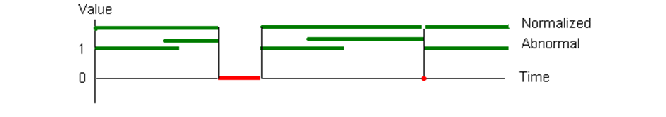
You might visualize a time condition as shown below. This illustrates the Boolean function of time concept. A time condition C is a function of time t, where C(t) is 0 or 1 for any t.
A time condition is true during specific time intervals, so it can be visualized as a set of line segments in one dimension (time). If condition C is defined by a set of time intervals, we interpret C(t) to be true when t falls on any one of the intervals, and false otherwise.

Here, the word "interval" means a segment of time with a defined start and stop time. The start time is included and the stop time is excluded. In other words, C(t) is true where t>=start and t<stop for any interval in the set which represents C. The word "duration" means a segment of time of a given length, but without a fixed start time. It is important not to confuse the use of the words "interval" and "duration."
A partitioned set is a special case where the end of each interval is the start of the next interval.

Although you might expect time conditions represented by partitioned sets to be true for all time, they actually become false and then return to true at the beginning of each interval. This provides a leading edge to trigger events.
A normal set does not have overlapping intervals. A set is abnormal when it has overlapping intervals. Abnormal sets are useful for defining complex time conditions as you will see later. However, the set for a complete time condition is normalized for interpretation as a Boolean function of time. The figure below illustrates how an abnormal set is normalized for condition interpretation. A condition is true at times included in any interval. When one interval starts at the stop time of another interval, the intervals are not combined. They only combine when the intervals overlap. Normalization will not alter a partitioned set.
Time functions provide common schedules based on the Gregorian calendar. These functions have names like year, month, day, hour, minute, and second. The time interval sets produced by these functions are what the names imply. The year time function returns intervals that start on January 1 at 00:00 and end on January 1 of the following year at 00:00. The month time function returns intervals that start on the first day of a month at 00:00 and end on the first day of the next month at 00:00. The day, hour, minute, and second time functions return an interval for every day, hour, minute, or second respectively.
Each of the functions described above produces a partitioned time interval set. Other time functions produce normalized time interval sets that are not partitioned. Examples are sunday, monday, ..., saturday, and january, february, ..., december. These functions produce time interval sets for a specific day of week or month of year. For example, the january function returns intervals that start on January 1 at 00:00 and end on February 1 at 00:00. The sunday function returns intervals that start on Sunday at 00:00 and end on Monday at 00:00.
The logical expression below contains a time condition using the day function. This could be used to trigger a rule every midnight when the ready variable is 1.
~(day) and ready=1
Time function parameters are used to select a subset of their intervals. For example, to specify only days 1, 15, and 28 of each month, a parameter list is specified for the day function. (See the section, Interval Selection Parameters.)
day(1,15,28)
Time expression operators are used to construct time interval sets based on other time interval sets. Some operators have a Boolean logic orientation. For example, when used in a time expression, and (&), or (|), and not (!) operate on time interval sets to produce new sets that behave in the same way separate time conditions would if combined using these same Boolean operators. The following logical expressions will have the same value at any given time.
     threshold=5 & ~(monday) & ! (~(january) | ~(june))
     threshold=5 & ~(monday&!(january|june))
Other operators are based purely on the notion of time interval sets. The figure below illustrates the union operation, which accepts any two sets, a and b, as operands and produces a new set (a,b). This condition includes the time intervals from both sets. (The union operator symbol is a comma.)

The union operator (,) is an example of an infix operator, meaning it is specified between two sets. Other operators, like ! (not), work on a single set. These operators are specified before the set and are called prefix operators.
A complex operator, [], enables indexed selection. The example below selects January 5.
day[5]january
As you can see, this operator accepts counters as parameters. In this case, the January function returns intervals representing the month of January for each year. The day function returns the 31 days of January. The indexed selection, [5], returns the fifth day of January.
These concepts are explained further in the sections that follow. However, you will find them easier to digest if you have an introductory understanding of the major concepts. So let's review quickly.
severity=9 and user="Fred" and ~(sunday)
          monday
          june
          quarter
day(5,19)
          (monday,wednesday,friday)
          friday[1]January
If a and b are time interval sets, a[n] b is a set of intervals selected from a, based on b. Specifically, for each interval of b, you select the nth overlapping interval of a.

The number n may be preceded by a minus sign (-) to reverse the direction of count. That is, a[-n]b selects the nth from the last overlapping interval of a for each interval of b.
Here are some examples of indexed selection using time functions as operands.
            day[1]month              first day of the month
            day[-1]month             last day of the month
            month[2]year             second month of the year
            day[62]year              sixty-second day of the year
            day[-3]year              3rd to last day of the year
Any number of indexes may be specified in an index list as illustrated below.
     	day[1,15,20]month
     	month[1,3,5,7,9,11]year
The result, as one you might expect, is to select every indexed interval. The comma (,) is referred to as the Union operator. The following schedules are identical.
     	day[1,15,20]month
     	(day[1]month),(day[15]month),(day[20]month)
A range specification is a shorthand notation for a list of consecutive indexes, where only the first and last index are given. The indexes between these values are "understood." The range symbol is two periods (..). The following schedules are identical.
     	day[1,2,3,4,5,10,11,12,13,14,15,16]month
     	day[1..5,10..16]month
Suppose you want to specify a schedule with intervals starting on the 1st day of the month and ending on the 16th day of the month. This could also be stated as the "1st through the 15th day of the month." The underscore character is used in this case.
day[1_15]month
You may combine simple indexes, index ranges, and spanned index ranges in a single index list.
day[1,3,10..17,18_20,25]month
Interval selection parameters are used similar to the indexed selection operator, [], introduced in the previous section. However, interval selection parameters use an implied function to perform selection. For example, day(1) specifies the first day of every month. In this case, the month function is implied.
The interpretation of selection parameters is inconsistent from function to function with respect to the base index and unit you are indexing, or indexing within. However, parameters generally conform to standard usage, so are relatively intuitive.
The indexed selection operator, [], provides a more consistent and flexible notation than selection parameters, so make use of indexed selection notation in the description of selection parameters. For review, if a and b are interval sets, then a[1]b specifies, for each interval of b, the first interval of a that overlaps the interval of b. The expressions below both return the first day of every month.
     	day(1)
     	day[1]month
The selection parameter notation is convenient because one of a or b is specified and the other is implied. For the "specific month of year" functions (jan(),feb(),mar(),...), you specify b, and a is understood to be day. The following schedules all specify the 15th of every January.
     	january(15)
     	day[15]january
     	day[15]month(1)
     	day[15]month[1]year
For functions other than "specific month of year" (jan(),feb(),mar(),...), you specify a, and b is understood. This is illustrated by the last two examples above, which show month(1) to be equivalent to month[1]year. In most cases, where a is partitioned, b is understood to be the partitioned schedule with intervals just larger than a. However, there are exceptions. In general, the translation from the convenient parameter notation to the consistent indexed selection notation is something one needs to learn. The column labeled "parameter(i)" in the following table describes this translation.
| Function | Abbr | Parent | Parameter(i) | Range of i
|
|---|---|---|---|---|
| millennium | - | millennium[i+1]Gregorian |
| |
| century | millennium | century[i+1]millennium |
| |
| decade | century | decade[i+1]century |
| |
| year | y | decade | year[i+1]decade | 0..9
|
| quarter | q | year | month[i*3-2_i*3]year | 1..4
|
| month | n | year | month[i]year | 1..12
|
| january | jan | year | day[i]jan | 1..31
|
| february | feb | year | day[i]feb | 1..31
|
| march | mar | year | day[i]mar | 1..31
|
| april | apr | year | day[i]apr | 1..31
|
| may | may | year | day[i]may | 1..31
|
| june | jun | year | day[i]jun | 1..31
|
| july | jul | year | day[i]jul | 1..31
|
| august | aug | year | day[i]aug | 1..31
|
| september | sep | year | day[i]sep | 1..31
|
| october | oct | year | day[i]oct | 1..31
|
| november | nov | year | day[i]nov | 1..31
|
| december | dec | year | day[i]dec | 1..31
|
| week | w | year | week[i]year | 1..54
|
| day | d | month | day[i]month | 1..31
|
| sunday | su | month | sunday[i]month | 1..5
|
| monday | mo | month | monday[i]month | 1..5
|
| tuesday | tu | month | tuesday[i]month | 1..5
|
| wednesday | we | month | wednesday[i]month | 1..5
|
| thursday | th | month | thursday[i]month | 1..5
|
| friday | fr | month | friday[i]month | 1..5
|
| saturday | sa | month | saturday[i]month | 1..5
|
| hour | h | day | hour[i+1]day | 0..23
|
| minute | m | hour | minute[i+1]hour | 0..59
|
| second | s | minute | second[i+1]minute | 0..59
|
Any schedule that can be specified using selection parameter notation can also be specified using indexed selection notation. However, the converse is not true. Indexed selection notation can be used to specify schedules that can not be specified in selection parameter notation. For example, selecting the 23rd Sunday of a year is straightforward using indexed selection. It is not possible to specify this schedule using selection parameters only.
su[23]year
Although you may avoid selection parameter notation without reducing the set of expressible schedules, where parameter notation can be used, it may be preferred for readability and efficiency.
     	jan(15)         is preferred over           day[15]jan
     	day(7)          is preferred over           day[7]month
Any number of parameters may be specified in a parameter list as illustrated below.
     	day(1,15,20)
     	january(24,25)
     	month(1,3,5,7,9,11)
The result, as you might expect, is to select every interval matching any of the specified parameters. The comma (,) is referred to as the Union operator. The following schedules are identical.
     	day(1,15,20)
     	day(1),day(15),day(20)
A range parameter is a shorthand notation for a list of consecutive numbers, where only the first and last numbers are given. The numbers between these values are "understood." The range symbol is two periods (..). The following expressions represent the same schedule.
     	day(1,2,3,4,5,10,11,12,13,14,15,16)
     	day(1..5,10..16)
Suppose you want to specify a schedule with intervals starting on the 1st day of the month and ending on the 16th day of the month. This could also be stated as the "1st through the 15th day of the month." The underscore character is used in this case.
day(1_15)
If a(x_y) represents (a[x] b)_(a[y] b) and x > y, then an interval of the set a(x_y) will start in one interval of b and stop in another interval of b. For the following example, intervals start on the 27th of one month and end on the 6th of the next month.
day(27_5)
You may combine simple parameters, range parameters, and span parameters in a single parameter list.
day(1,3,10..17,18_20,25)
If a(1) is shorthand for a[1] b, then b is the parent function of a. For example, month is the parent of day, and year is the parent of month. With this understanding, you can specify parameters for b in a parameter list for a. The following expressions specify every January 5th and October 11th respectively.
     	day(1/5)
     	day(10/11)
Again, it is helpful to describe this notation in terms of indexed selection. The following expressions represent the same schedules as the expressions above.
            day[5]month[1]year
            day[11]month[10]year
Use of parent parameters is not limited to one level. The following set of equivalent expressions illustrates this concept.
            minute(1999/12/24@11:00)

            minute(11:00).day(1999/12/24)
            minute(11:00).day(24).month(1999/12)
            minute(11:00).day(24).month(12).year(1999)
            minute[1]hour[12]day[24]month[12]year(1999)
The previous example defined a specific minute in time. There is only one interval in the resulting set. Suppose you wanted to schedule one hour at noon on every April 15th. This is accomplished by simply not specifying a year.
     	hour(4/15@12)

     	hour(12).day(4/15)
     	hour(12).day(15).month(4)
     	hour[13]day[15]month[4]year
The following convention is used for parent parameter separators.
     No separator: millennium, century, decade, year

            year(2010)

     year/month/day@hour:minute:second

     day(2005/1/15)          day(15).month(1).year(2005)
     month(2006/7)           month(7).year(2006)
     hour(1/25@10)           hour(10).day(1/25)
     hour(5@11)              hour(11).day(5)
     minute(1/25@10:42)      minute(10:42).day(1/25)
     minute(12:17)           minute(17).hour(12)
     minute(15@12:17)        minute(17).hour(12).day(15)
     second(12:17:52)        second(52).minute(12:17)
     second(5@12:17:52)      second(52).minute(12:17).day(5)

     Uncommon parent parameters.
     sunday(1/3)             sunday(3).jan
     january(2006/15)        day(2006/1/15)
     quarter(1/3)            quarter(3).year(1)
     week(1/27)              week(27).year(1)
The "specific month of year" functions (jan, feb, mar, ...) are an exception that require special attention. The base parameters select days within the specific month, but the parent function is year. You should avoid using parent parameters when the meaning is not clear.
Range and span parameters specify a first and last parameter for a series of consecutive intervals within a schedule. Parent parameters may be used in either or both of the ends.
     hour(4/15@12_17)        hour(12_17).day(4/15)
     hour(4/15@12_16@12)    (hour(12).day(4/15))_(hour(13).day(16))
     hour(15@20_12@5)       (hour(20).day(15))_(hour(6).day(12))
This section describes all 30 time functions. Time functions produce time interval sets based on the system clock and routines provided by the host environment. There are 11 partitioned time functions: millennium, century, decade, year, quarter, month, week, day, hour, minute, and second. Except for the first three, which are seldom used, time functions have single character abbreviations (y, q, n, w, d, h, m, s). The other 19 schedule functions select specific intervals from the partitioned sets, that is, months of the year and days of the week. These functions have three and two character abbreviations.
There are defects and limitations associated with these functions. The year function without parameters is reliable. Avoid millennium, century, and decade, and do not use parameters with the year function until the defects have been fixed.
A time function is defined for each of the digits of a four digit year. Typically, millennium, century, and decade are specified as parent parameters to year.
year(2003)
| Function | Abbr | Parent | Boundary
|
|---|---|---|---|
| millennium | - | First second of millennium
| |
| century | millennium | First second of century
| |
| decade | century | First second of decade
| |
| year | y | decade | First second of year
|
The examples below specify equivalent schedules. (The current implementation does not support these examples. No schedule greater than January 2038 can actually be represented in the internal UTC format used by NodeBrain.)
     	millennium(3)
     	century(30_40)
     	decade(300_400)
     	year(3000_4000)
The breakout of each digit of a year is a bit strange perhaps, but it provides some flexibility that you would not have it you had a single year function. If you don't specify the parent parameters by using all four digits, you select only on the specified digits.
     	year(0,2,4,6,8)		Even years
     	year(1,3,5,7,9)		Odd years

     	year(0_9)               Same as decade
     	year(00_99)             Same as century
     	year(000_999)           Same as millennium
A year is divided into the standard 12 months selected using the month function. Specific months may be selected using the function named for the month (january, february, march, ..., ...december). The year is also divided into four three-month quarters selected using the quarter function.
| Function | Abbr | Parent | Boundary
|
|---|---|---|---|
| quarter | q | year | 1st second of Jan., Apr., Jul., Oct.
|
| month | n | year | 1st second of month
|
| january | jan | year | " [selection parameter is day]
|
| february | feb | year | "
|
| march | mar | year | "
|
| april | apr | year | "
|
| may | may | year | "
|
| june | jun | year | "
|
| july | jul | year | "
|
| august | aug | year | "
|
| september | sep | year | "
|
| october | oct | year | "
|
| november | nov | year | "
|
| december | dec | year | "
|
The examples below show the relationship between quarter and month.
     	quarter(1)		month(1_3)
     	quarter(2)		month(4_6)
     	quarter(3_4)		month(7_12)
Year is the parent schedule for all of these functions.
     	quarter(2005/3)         quarter(3).year(2005)
     	month(2009/7)           month(7).year(2009)
     	january(2007/15)        january(15).year(2007)
     			        day(2007/1/15)
Notice the strange case of individual months like January. The parent schedule is year, but the intervals are days, like the day function. The calendar month functions are more intuitive when a year is not specified.
jan(15), jun(6), oct(11)
The day schedule function returns 24-hour intervals corresponding to days of the Gregorian calendar. The week function returns 7-day intervals corresponding to weeks of the Gregorian calendar. The individual days of a week are returned by the functions cleverly named sunday, monday, tuesday, wednesday, thursday, friday, and saturday.
| Function | Abbr | Parent | Boundary
|
|---|---|---|---|
| week | w | year | 1st second of Sunday
|
| day | d | month | 1st second of day
|
| sunday | su | month | "
|
| monday | mo | month | "
|
| tuesday | tu | month | "
|
| wednesday | we | month | "
|
| thursday | th | month | "
|
| friday | fr | month | "
|
| saturday | sa | month | "
|
The parent schedule for week is year, while the parent of day and sunday through saturday is month.
     	week(20)        20th week overlapping each year   -  week[20]year
                             To get 20th full week, use "w.su[20]year".
     	day(15)         15th day of each month
     	tuesday         Every Tuesday
     	saturday(3)     3rd Saturday of each month
The hour, minute, and second functions are used to specify time intervals within a day. The day schedule is the parent of hour, which is the parent of minute, which is the parent of second.
| Function | Abbr | Parent | Boundary
|
|---|---|---|---|
| hour | h | day | 1st second of hour
|
| minute | m | hour | 1st second of minute
|
| second | s | minute | Every second
|
     	hour(7)                 8th hour of every day. (07:00 to 08:00)
     	hour(15@7)             7:00 to 8:00 on the 15th of each month
     	minute(5)               6th minute of every hour
     	minute(7:45)            07:45 to 07:46 every day
     	second(0:10)            11th second of every hour

     	s(5).m(30).h(10)        10:30:05 to 10:30:06 every day
     	s(10:30:05)             10:30:05 to 10:30:06 every day
Time interval sets can be transformed into new sets using the prefix operators described in this section.
| Syntax | Operation | Description
|
|---|---|---|
| =a | Conflict | Intervals of a that intersect other intervals of a.
|
| |a | Connect | Combine connecting (end = start) intervals and overlapping intervals.
|
| #a | Partition | Partition time from interval start to interval start.
|
| !a | Not | Inverse schedule has intervals filling gaps not covered by any interval of a.
|
| &a | Overlap | Intervals generated for times covered by more than one interval of a.
|
| ~a | Normal | Combine overlapping intervals of a.
|
| %a | Unique | Intervals generated for times covered by one and only one interval of a.
|
The conflict operator (=) selects intervals of a set that intersect other intervals of the set. If the intervals of the original set represent meetings you would like to attend, this operation produces a set of conflicting meetings.
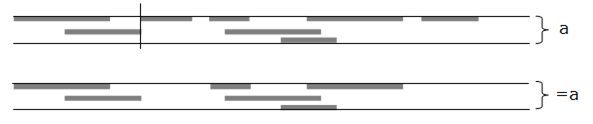
The connect operator (|) combines intervals where the end of one is greater than or equal to the start of another. In other words, it combines overlapping and successive intervals.
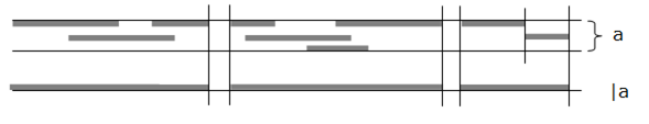
The partition operator (#) generates a partitioned set using the start of each interval in the operand set.
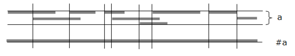
The not operator (!) generates a set with intervals that fill the gaps not covered by any interval of the operand set.
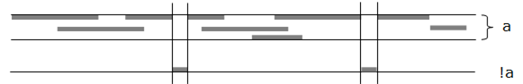
The overlap operator (&) generates intervals covered by more than one interval in the operand set.
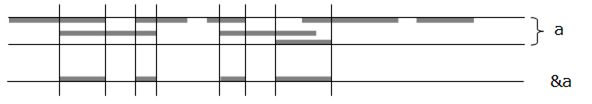
The normalize operator (~) combines intervals that overlap, but retains successive intervals. This operation is always performed on a time expression used in a time condition "~(time_expression)", so you only need to specify it when you want to normalize sub-expressions.
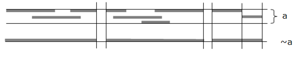
The unique operator (%) generates intervals covered by one and only one interval of the operand set. It preserves non-overlapping edges.
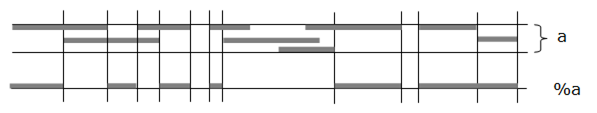
Time condition operators are used in expressions to build new interval sets from the output of time functions and other time expressions. The infix operators, described in this section, perform operations on two sets. The operator is specified between the sets as shown in the examples below.
     	sunday.january          Sundays of January
     	day!tuesday             Any day except Tuesday
Many of the operator symbols are used as both infix and prefix operators. If $ were an operator symbol, it would be nice if you could say "$a" is the same as "a$a". In some cases (e.g., | and #) this would be a true statement. In others, it clearly isn't. For example, "!a" is not the same as "a!a". However, there is always some similarity in infix and prefix operations represented by the same symbol. For example, !, &, and | are always somehow reminding us of Boolean Not, And, and Or.
| Syntax | Operation | Description
|
|---|---|---|
| a,b | Union | Union of intervals from a and b
|
| a.b | Selection | Intervals of b that intersect intervals of b
|
| a!b | Rejection | Intervals of a that do not intersect intervals of b
|
| a#b | Until | Intervals of a with lengths adjusted to the nearest start of an interval of b
|
| a&b | And | True when both a and b are true
|
| a|b | Or | True when a or b are true
|
| a%b | Xor | True when a or b, but not both, are true
|
The union operator (,) produces a set containing all intervals found in either of the two operand sets. Intervals found in both operand sets are found only once in the resulting set. In other words, duplicates are not produced.
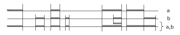
The selection operator (.) selects intervals from the first operand set that intersect intervals of the second operand set.
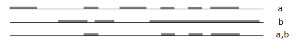
The rejection operator (!) selects intervals of the first operand set that do not intersect intervals of the second operand set.
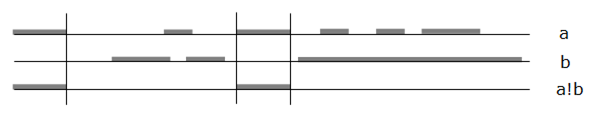
The until operator (#) extends the end of intervals of the first operand set to the next start of an interval of the second operand set.
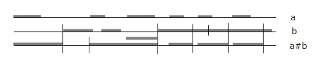
The and operator (&) produces a set of intervals where both operand sets are true.
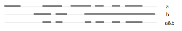
The or operator (|) produces a set of intervals where at least on of the operand sets is true.
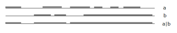
The exclusive or operator (%) produces a set of intervals where one of the operand sets is true, but not both.
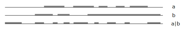
Syntax
|
A time sequence is a method of generating a time interval set by stepping through time and setting values of true and false. The following example is interpreted as "true for 2 days, false for 1 day, true for 3 days and false for 1 day."
{/2d\d/3d\d}
A time sequence, by itself, starts from the time it is translated by the interpreter. If this example were used in a cell condition translated at 15:43 on a Saturday, the 8th of some month, the resulting time interval set would be aligned to that time.
            forecast ~{/2d\d/3d\}

            sa yyyy/mm/08 15:43 - mo yyyy/mm/10 15:43
            tu yyyy/mm/11 15:43 - fr yyyy/mm/12 15:43
A time sequence can be aligned to the intervals of another set using the select operator (.). The following schedules are the same.
            ~({/2d\d/3d\}.n)
            ~(d[1_2,4_6]n)
A recurring event at any time of day can be schedule for a specified duration. This example is specifies a 2 hour and 10 minute event starting at 17:10 on the fifth of each month.
~({/2h10m}.m(17:10).d(5))
You can also specify a repeating time sequence within a time sequence. This example specifies 4 hours on and 4 hours off indefinitely.
~{*{/4h\4h}}
Intervals of a repeating time sequence are selected by (and aligned to) another time interval set just like a non-repeating time sequence. The following example specifies 4 hours on and 4 hours off during intervals of 2 days on and 2 days of during each monthly interval.
~({*{/4h\4h}}.{*{/2d\2d}}.n)
Time sequences can be repeated a finite number of times also. This example repeats a strange pattern 5 times.
~{5{/2h\1h/3m\2m}}
Further nesting is allowed.
~{3{5{/2h\1h/3m\2m}2{/1d\2d2{/1h\2h}}}}
Commas may be used if you like.
~{3{5{/2h,\1h,/3m,\2m},2{/1d,\2d,2{/1h,\2h}}}}
Negative numbers may be used on steps, but not repeat counts. Here you step 1 month less 7 days and then start 5 segments of 1 month each.
~{1n-7d,5{/1n}}
It is not necessary to specify a plus (+), but it is allowed. The following schedules produce the same results.
     	~({/2h+30m}.h(8))
     	~({/2h,30m}.h(8))
     	~({/2h30m}.h(8))
When specifying a partitioned set, the false state (\) is assumed at the end of each specified interval.
~{*{/1n/2n/2n/1n}}
Syntax
|
For monitoring applications, you often just need a simple repeating schedule of a specific duration. For that, there is a simplified syntax. The following schedules produce the same results.
     ~(15m)           Pulse condition

     ~{*{15m/}}   Time sequence
A pulse conditions resolves to a single number of seconds. For example, "2h1m3s" resolves to 7263 seconds. The value of a pulse condition is not true until the duration is complete. It then remains true, except for the last second of every duration. This provides a leading edge to trigger rule conditions.
Here you see a simple rule to run a script every 10 minutes. The script will run for the first time 10 minutes after the rule is defined.
define myRule on(~(10m)):=/home/fred/bin/myscript.pl
A rule associates an action with a condition. It tells the rule engine what to watch for and what to do if it sees it. In English, you might express a rule using a sentence of the form "If condition, then action." For example, "If it starts to rain, then go inside the barn." NodeBrain supports commands with similar structures.
     define term type(condition) action;                                     [Simple rule]
     {type(condition);action;type(condition);action; }     [Sequence rule]
Simple rules constantly watch for the specified condition and take the specified action when the condition is true. These rules have defined names that can be used to reference the rule.
     define term type(condition) action;

     define r1 if(a=1 and b=2) c=3:
     define r2 on(a=2 and b=1) c=7.5;
     define r3 when(a+b=9) ?c :=/home/fred/niner.pl;

     disable r1;     # This prevents rule r1 from responding to the condition
     enable r1;      # This causes rule r1 to start responding again
     undefined r1;   # This removes r1 from the engine's memory
The different types of conditions (if, on, or when) provide for different behavior.
| Type | Behavior
|
|---|---|
| if | Only responds to an alert to the context in which the rule is defined. Responds when the condition is true, even if it was already true. This is used for event monitoring.
|
| on | Responds to any assert or alert that transitions the condition to a true state. This is used for state monitoring.
|
| when | Like on, but is automatically undefined when the condition transitions to true for the first time. This is a one-time rule. As such, it can be used for either event or state monitoring.
|
The action for simple rules may be a compiled assertion or a command that is interpreted each time the rule fires.
     define term type(condition) [assertion] [:command | ; ]

     define r0 on(a=7);              [no action]
     define r1 on(a=1) b=2;          [assertion only]
     define r2 on(a=3):-dir          [command only]
     define r3 on(a=5) b=3:-dir      [assertion and command]
You can group a set of rules within the context of a node. Normally when you have a large number of rules you can organize them into smaller sets by using multiple nodes. For example, suppose you are monitoring 5 servers. The rules for a single server might look something like this.
     define server node;
     server. define 'myhost1.enterprise.com' node;
     server.'myhost1.enterprise.com'. define r1 on(!.pingable) action11;
     server.'myhost1.enterprise.com'. define r2 on(cpu>95) action12;
     server.'myhost1.enterprise.com'. define r3 on(disk>80) action13;
You might have different rules for each server, organized by creating a node for each one.
     server. define 'myhost2.enterprise.com' node;
     server.'myhost2.enterprise.com'. define r1 on(disk>80) action21;
     server.'myhost2.enterprise.com'. define r2 on(cpu>92) action22;
If you find the rule sets for each server are similar, they may be easier to maintain if you create a single source file a server rule set and source the file for each server.
     # Source File: Server.nb
     #--------------------------
     %default name="oops",ping=1,disk=80,cpu=95
     %if(ping);
     server.'%{name}'. define r1 on(!.pingable) action1;
     %endif;
     server.'%{name}'. define r2 on(cpu>%{cpu}) action2;
     server.'%{name}'. define r3 on(disk>%{disk}) action3;

     # Main rule file
     #==================
     source server.nb,name="myhost1.enterprise.com";
     source server.nb,name="myhost2.enterprise.com",cpu=92
     ...
In this example, you have been assuming the various elements of state associated with each server are updated independently as shown here.
     assert server.'myhost1.enterprise.com'.disk=82;
     assert server.'myhost2.enterprise.com'.cpu=64;
     assert !server.'myhost1.enterprise.com'.pingable;
You are also assuming that you may have rules with conditions based on more than one variable for a given server or for multiple servers. And, finally, assume you may have different thresholds for each server. When these assumptions are true, you need to maintain the state of all parameters for each server. If these assumptions are not true, you can simplify the rule set by creating just one set of rules for all servers.
     define server node;
     server. define r1 on(!pingable) action1;
     server. define r2 on(cpu>95) action2;
     server. define r3 on(disk>80) action3;
With this set of rules, assertions might look like this. Notice that the server name is available to be used via symbolic substitution in the rule actions.
     server. assert name="myhost1.enterprise.com",disk=82;
     server. assert name="myhost2.enterprise.com",cpu=64;
     server. assert name="myhost1.enterprise.com",!pingable;
Depending on how you collect the variable values, it may be convenient to report all of the variables at once.
server. assert name="myhost1.enterprise.com",disk=82,cpu=95,pingable;
In this case, you can once again introduce compound conditions based on multiple parameters for a given system.
server. define r4 on(disk<20 and cpu<10) action4;
You may notice you are slowly converting this application from a state monitoring system into an event monitoring system. By doing this you have created two new problems. First, the rules fail to respond to a problem on a given server when the same problem existed for the server that reported previously. Remember, on rules only fire when the condition transitions to True. So you need to change the rules to if rules and use alert instead of assert.
     define server node;
     server. define r1 if(!.pingable) action1;
     server. define r2 if(cpu>95) action2;
     server. define r3 if(disk>80) action3;

     server. alert name="myhost1.enterprise.com",disk=82;
     server. alert name="myhost2.enterprise.com",cpu=64;
     server. alert name="myhost1.enterprise.com",!pingable;
Second, the system has become chatty. The rules will respond over and over when you get continued reports of a problem. You can solve this by including some cache nodes.
     define server node;
     server. define cPing node cache:(~(20m):server);
     server. define cCpu node cache:(~(2h):server);
     server. define cDisk node cache:(~(4h):server);

     server. define r1 if(!cPing(server) and !.pingable) cPing(server): action1;
     server. define r2 if(!cCpu(server) and cpu>95) cCpu(server): action2;
     server. define r3 if(!cDisk(server) and disk>80) cDisk(server): action3;
Now the rules will only take action every 20 minutes on ping problems, 2 hours for high cpu utilization, and 4 hours for high disk space utilization. This is good, but what if a problem is resolved and then returns within this interval. For example, let's say for action3 you open a trouble ticket for an SA to clean up the disk space and the SA gets it down to 70% used within 90 minutes and closes out the ticket. If the usage goes above 80% again within the 4-hour cache interval, the new problem will not be detected. This can be solved by adding another rule with a reset threshold.
     server. define r3On if(!cDisk(server) and disk>80) cDisk(server): action3;
     server. define r3Off if(cDisk(server) and disk<75) !cDisk(server);
These two rules work in combination like a flip-flop condition you might elect to use for state monitoring with rules for each server.
server. define r3 on(.disk>80 ^ .disk<75): action3;
This is fine, but if the only action is to issue an alarm, you can create an alarm cache node and let it handle the deduplication. Then you can go back to the simple set of rules.
     define server node;
     server. define r1 if(!.pingable):alarm. alert ("message1");
     server. define r2 if(cpu>95):alarm. alert ("message2");
     server. define r3 if(disk>80):alarm. alert ("message3");
See Appendix C, section C.1 Sample Alarm Script, for an example of what the alarm cache node might look like.
Another type of rule, when, can be used in situations when you want to detect a condition one time only. This can be used for both state and event monitoring.
     define r1 when(a=1 and b=2):=/home/me/script.pl

     assert a=1,b=2; # causes r1 to fire and undefined itself
       -or-
     alert a=1,b=2;
For a real world example, let's assume you have a trouble ticket system with an interface that returns a ticket number when you open a new ticket, and an interface to close a ticket by number. A rule to generate a ticket might look like this.
     define r1 on(condition)\
       :=$ ticketGenerationScript "closeCondition" "ticketInfo"
     define ticket node;
Your ticket generation script could generate a ticket and define a when rule to monitor for the condition used to close the ticket.
ticket. define 'ticketNumber' when(closeCondition):=ticketCloseScript "..."
It is also possible to use when rules that create when rules that create when rules, and so on, to monitor for a sequence of conditions. The next section describes sequence rules as an alternative to this approach.
Warning: This feature is experimental and should not be considered stable. Significant changes may occur prior to version 1.0.
Syntax: Superset of time sequence
|
A sequence rule provides an alternative to simple rules and state variables as a way to recognize a sequence of events and take actions at various points within the sequence. There are two goals: (1) processing efficiency and (2) coding efficiency.
     	define r1 on(state=1 and A=5) state=2: command1
     	define r2 on(state=2 and A=7) state=3; command2
     	define r3 on(state=3 and A=9) state=1;
{*{on(A=5): command1;on(A=7): command2;on(A=9) }}
A sequence rule can be more efficient to process because it automatically enables and disables rule conditions, watching only for those conditions that support a transition to the next state in the sequence. In the example above, the simple rules are always monitoring for three values of the state variable and three values of A. When one of these relational conditions transitions to True, the Boolean "and" condition must be re-evaluated. The equivalent sequence rule only monitors for one relational condition at a time. It first monitors for A=5. When this condition transitions to True, the condition is disabled and command1 is interpreted. Next, the relational condition A=7 is enabled. When it transitions to True, the condition is disabled and command2 is interpreted. Next, the condition A=9 is enabled. When True, it is disabled and it loops back to enable A=5.
Coding efficiency is the second goal. One aspect of this is illustrated by the example above. You are able to use one rule instead of three, and you don't have to mess with the state variable. However, there are other advantages to sequence rules. Because a sequence rule supports local variables, it is easier to avoid naming conflicts by using local variables that are not exposed to all rules like context terms. In the following example, when A=5 the value of B is captured as %b (local variables start with "%"). This variable is then used in the second condition.
{*{on(A=5)`%b=B: command1;on(A=%b+2): command2;}}
Sequence rules are not named. This may be convenient in situations where you have rules that generate rules.
     define watching node cache:(x);
     define r1 if(A=1 and !watching(B)): \
      {`watching(B),%b=B;on(A=7 and B=%B)`!watching(%b);: command;}
     alert A=1,B=2; # spin off sequence rule for B=2 - new thread
     alert A=2,B=4;
     alert A=1,B=2;
     alert A=1,B=3; # spin off sequence rule for B=3 - new thread
     alert A=7,B=3; # interpret command with %b=3
     alert A=7,B=2; # interpret command with %b=2;
     alert A=1,B=2; # spin off sequence rule for B=2 - new thread
Although this is a trivial example, it illustrates the general idea. You want to be able to recognize a condition and start a new monitoring thread based on specific attributes. For this example, you can use two simple rules to accomplish the same thing.
     	define watching node cache:(x);
     	define r1 if(A=1 and !watching(B)) watching(B);
     	define r2 if(A=7 and watching(B)) !watching(B):command
But if you add a little more complexity to this problem, it becomes more difficult with simple rules. Suppose an event attribute C provides the value of A you want to watch for.
alert A=1,B=2,C=5; # we want to watch for (A=5 and B=2)
In this case, you might want to use a sequence rule.
     define watching node cache:(x);
     define r1 if(A=1 and !watching(B)): ...
        {`watching(B),%b=B,%c=C; ...
           on(A=%c and B=%B)`!watching(%b);:command;}
With increasing numbers of key event attributes and steps in the sequence you need to monitor, you expect the use of sequence rules to reduce the dependence on cache nodes and state variables to maintain state. This should reduce the number of rules and the complexity of simple rule conditions.
Now let's look at the individual statements within a sequence rule.
     Syntax:	`assertion;

     Example:	`a=1,b=2;
The sequence assert statement is simply an assert command using the backtick shorthand for the verb and terminated with a semi-colon.
     Syntax:	:command;

     Example:	:myCache. alert ("abc");
A sequence command statement can be any valid interpreter statement delimited by a semi-colon. This is somewhat restrictive because valid commands may contain semi-colons. You can get around this using delayed symbolic substitution. (In a future release, we plan to have built-in variables for this purpose.)
     	define semi cell ";";
     	{on(cond1);:$ =script1.pl abc$${semi}script2.pl;on(cond1);...}
     Syntax:	=cellExpression;
     		/
     		\

     Examples:	=5;
     		=a+b;
Publishing a value for a sequence is useful when a sequence is used within a cell expression. In the following example, the sequence takes on an initial value of 5 and then alternates between 3 and 4 based on the transition of A to 2 and a 10 minute timer.
     	assert X=={=5;*{onif(A=2);=3;10m;=4}}+B;
     	define r1 on(X=3 and Y>7) action;
When the sequence publishes a new value, the expression {...}+B is re-evaluated and the new value is published to X, causing re-evaluation of X=3 and potentially the AND condition in r1.
Because a sequence is a superset of a time sequence, you may use / and \ as shorthand notation to publish 1 and ! respectively.
     	/	same as	=1;
     	\	same as =!;
     Syntax:         (timeExpression)
                     timeInterval

     Example:        (mo,we,fr)      [wait until next Monday, Wednesday, or Friday]
                     (m(45))         [wait until 45 minutes after the hour]
                     10s             [wait 10 seconds]
The wait statements are the same as in a time sequence. (See Chapter 5, Time Conditions.)
     Syntax:         on(condition);
                     onif(condition);

     Examples:       on(a=1 and b=2);
                     onif(a=1 and b=2);
The on and onif statements block execution of a sequence thread until the specified condition is True (onif) or transitions to True (on). If the condition is already True when the statement executes, onif will not block, and on will block until the next transition to True.
     Syntax:         if(condition) statement; [else statement;]

     Examples:       if(a=1)`b=2;
                     if(a=1)`b=2;else`b=7;
                     if(a=1) {`b=2;show -t; }else{`b=7;cSystem. assert (system);}
The if statement is similar to that in your favorite high level language. You should not confuse the if statement with simple if rules. The if statement does not wait for a condition to be True and has no relationship to the alert command.
     Syntax:         { integer | * } {...}

     Examples:        5{(mo);on(a=2):myscript.pl; }
                      *{on(a=3):myscript.pl; }
The repeat statement is used to perform a subsequence a specific number of times or forever (*).
There are several deficiencies in the current implementation of the sequence rule. Some that we intend to resolve in a future release are listed here.
WHILE or UNTIL statement
if rule for event monitoring
on statement (blocking SWITCH statement)
exit statement
We elected to leave sequence rules unfinished in release 0.6.0 because they were not a priority for this release and we have been unable to devote sufficient time to complete the release in a reasonable period. Delaying the release further was not a good alternative.
All commands conform to a common general syntax.
Syntax
|
A command may start with a context prefix that tells the interpreter the context in which to interpret the command following the prefix. A context prefix is a context identifier ending with a period. Every term of a context identifier must be defined as a node. In the following sample code, the context prefixes are shown in bold font.
             define kinda node;
             kinda. define really node;
             kinda.really. define solar cell;
A node command also starts with a context identifier, but the identifier is followed by a left parenthesis or a colon, and the identifier must be defined with a skill. Using a skill named "magic", it might look like this.
     	define kinda node;
     	kinda. define really node magic;
     	kinda.really:This is a message to the magic skill
     	kinda.really(4,"sure"):This is a message to the magic skill
When a context identifier starts with the at symbol (@), the context is qualified starting at the top level.
Commands starting with verbs are described in the remainder of this chapter and those starting with special symbols are described in the next chapter.
The alert command is used to report an event to a set of rules defined within the context of a node.
Syntax
|
When an alert command is received by the interpreter, the specified assertions are made from left to right. In the following example, the cell identified by the term A is assigned the value of 3*5, and then the cell identified by the term B is defined to have the value of A+4, and finally A is assigned the value of 3. At the completion of these assertions, A=3 and B=7==A+4.
alert A=3*5,B==A+4,A=3;
Once the specified, assertions have been made, the interpreter re-evaluates any cell that references a changed cell. The following rule condition references cells that reference A and B and must be re-evaluated when their values change.
define r1 on(A>2 | B=4);
When the value of a cell remains the same, dependent cells are not re-evaluated. This alert command would not cause re-evaluation if it followed the previous alert command because the value of A is still three and value of B is still 7.
alert A=3,B==2*A+1;
When cell evaluation is complete, the interpreter takes the actions specified by defined rules. Any on or when rule whose condition transitions to true (from false or unknown) will fire. In addition, any if rule defined in the node that is the context of the alert command, whose condition is true, will fire, even if it was already true before the alert.
True if rules defined in other nodes will not fire, even if the alert command makes assertions to terms within those nodes
that make the if rules true.
An alert command will only trigger if rules in the node to which it is directed by the command context prefix.
You can think of an alert command as a representation of an event. The assertion provides event parameters. Rules within the alerted context (normally if rules) determine the response.
An alert command does everything an assert command does, but has two additional features. The first is the activation of if rules as described above.
The second is a notion called "alert attribute transience". This means simple terms asserted within the context node by an alert command are
assumed to be event attributes and will revert to Unknown if not specified on the next alert to the same context node. This does not apply to terms
defined in other nodes, even subordinate nodes. Nor does it apply to node function call assertions.
The purpose of this feature is to enable an alert to include both event and state intended assertions. State intended assertions are
preserved by directing them to a different node, or by simply being node function assertions. Event intended assertions are
made to terms in the context node (target of the alert), and are reset to Unknown when not specified on a subsequent alert.
This ensures that rules are responding only to the event attribute values of the current alert.
In a special case, this might include the ability to respond to the absence of a known value for an event attribute on the current alert—by monitoring
for the Unknown value.
In the example below, a is intended as a state term, while x.b and x.c are intended as event terms. Because x.c is not specified
on the second alert, it reverts to Unknown. Because a is not within the alert context, it does not revert to Unknown.
     define a cell ?;
     x. define r1 if(a=1 and .b=2 and .c=3);
     x. alert a=1,b=2,c=3;  # this will cause rule r1 to fire
     x. alert b=2;          # this will not because a=1,b=2,c=?
If the alerted node has the skill to accept assertions (i.e., a cache), you may specify one or more node function calls by simply providing an argument list. The second line below does the same as the first, but the inclusion of the node function symbol @ may make it more clear that a node function is being invoked to perform an assertion. The third line below uses a different node function of the same node to address a different facet of the node.
     alert ("goofy","silly"),A=3,B=4;
     alert @("goofy","silly"),A=3,B=4;
     alert @foo("goofy","silly"),A=3,B=4;
Using alert arguments with a cache node is useful for establishing thresholds that prevent a duplicate action within some interval of time.
     	define hostUserType node cache:(~(1h):host,user,type(1));
     	hostUserType. define r1 if(type._hitState): action
Given the node definition above, the following alert could repeat frequently without triggering more than one action per hour.
hostUserType. alert ("goofy","sally","HttpGet"),text="...";
Actually, if the alert repeated continually and the time between alerts was always less than 1 hour, the action would never repeat. This is because the counter would never fall to a reset value. You could ensure at least one action every three hours by scheduling a reset of the entire cache.
hostUserType. define r0 on(~(3h)):assert ?();
The first alert for any given cache row following the reset would now cause the action to trigger. This would be in addition to an action following any 1 hour interval during which the event did not occur.
A cache is used as an example here, but assertions can be used for any node whose module supports assertions.
The archive command is used to archive the current log file.
Syntax
|
Although an archive command may come from an external source on demand, normally an agent will have a scheduled time that it archives the log file. The following rule will cause a daily archive at midnight.
define r0 on(~(0h)):archive
The name of the log file must be set.
set log="/var/log/goofy.log";
When the archive command is issued, nb renames the current log file by inserting the time YYYYMMDDHHMMSS and creates a new one.
     	/var/log/goofy.20030118000000.log       # archived log
     	/var/log/goofy.log                      # new current log
The assert command is used to report a state change. The syntax is identical to the alert command, except for the verb. A backtick (`) is used as a shorthand notation for assert.
Syntax
|
Unlike the alert command, the assert command does not directly trigger IF rules. Both commands trigger on and when rules when their condition transitions to a true state (from false or unknown).
assert A=1,B=2,C,!D;
The assertion above would cause the following rule to trigger if the condition was not already true. (Note: C=1 and D=!.)
define r1 on(A=1 and B=2 and C and !D): action
The addressed context will be used implicitly for node assertions where you leave off the node name. In the example below, "connie" is assumed in the first assertion within the list, while "job" is specified explicitly in the last assertion within the list.
     	define job node tree;
     	define connie node cache:(x,y,z);

     	connie. assert ("huey","duey","louie"),A=1,B=2,job("salesman");
A cache row is deleted by asserting it to be "unknown" using a question mark (?), or false using (!). They perform the same function here because a cache uses the "closed world" assumption—if it is unknown, it is false.
connie. assert ?("huey","duey","louie"),A=1,B=2;
Multiple rows may be deleted by negating a partial row specification.
     	connie. assert ?("huey","duey"),A=1,B=2;
     	connie. assert ?("huey"),A=1,B=2;               # delete any row starting "huey"
     	connie. assert ?(),A=1,B=2;                     # delete all rows
The way a node handles assertions depends on the node module providing the functionality. A cache is used as an example here, but other node modules will implement different behavior.
Refer to Cell Evaluation in Chapter 1 for an explanation of how the interpreter responds to assertions.
The declare statement is used to name special objects in a name space unique to the object type.
Syntax
|
These objects play a special configuration role, and their names should not be confused with terms used in cell expressions. Declared terms are global, so you may reference them in commands interpreted in any context.
A NodeBrain identity is similar to the familiar notion of a user account for applications and operating systems. Commands execute with the permissions of the active identity, which by default is an identity named "default."
Syntax
|
Node modules that accept commands from external sources (e.g., peer) must specify the active identity when issuing commands to the interpreter and are fully responsible for identity authentication. This allows for a wide variety of authentication mechanisms while providing a common authorization mechanism. The peer module uses a public/private key authentication technique for socket connects, while peer queues and the pipe module rely on standard file permissions. The Webster module uses x509 certificates or fixed passwords. Although there are no current examples, a module could use one-time password authentication.
Sets of permissions are associated with identity ranks, which are similar predefined user groups with static permissions. An identity's rank defaults to "guest" if not specified. Use the rank command to change the rank of an identity.
See the rank command for information on permissions.
Calendars are declared for reference in time expressions. This is done to simplify time expression coding or provide a single point of change for common time conditions.
Syntax
|
A calendar is specified with a single time expression as illustrated by the following example.
declare Dayoff calendar friday[-1]month; # last Friday of month
Like all declared terms, calendar terms are managed in a separate name space and are available for use within time expressions in any context. Within a time expression, declared calendars are recognized by an uppercase letter. The following rules have equivalent conditions given the previous declaration of "Dayoff".
     	define r1 on(a=1 and ~((monday,wednesday,friday)!Dayoff));
     	define r2 on(a=1 and ~((monday,wednesday,friday)!(friday[-1]month));
The following time condition specifies the Tuesday of the week of a Dayoff.
tu.w.Dayoff
Once declared in a NodeBrain process, calendars may not be modified. A change to a calendar requires a process restart.
Modules are declared to help NodeBrain locate them or to specify special initialization parameters. If NodeBrain is properly installed, you will not need to declare modules under normal conditions.
Syntax
|
If you are declaring a module only to help NodeBrain locate it, you may declare the path only. The term is used as the identifier to formulate the filename. The following examples are equivalent on a platform that uses *.so as a module suffix. The first option has the advantage of being platform independent.
     	declare snmptrap module {"."};

     	declare snmptrap module {"."}snmptrap;

     	declare snmptrap module ./nb_snmptrap.so;
The last example above does not allow for a path list. NodeBrain will look only in the current directory. The following examples specify multiple directories to search in sequence.
     	declare snmptrap module {".:..:/home/fred"};
     	declare snmptrap module {".:..:/home/fred"}mysnmptrap;
If you don't specify a path list or a path as part of the filename, the native system search path applies. You can often control this with a platform-specific environment variable like LD_LIBRARY_PATH. NodeBrain also allows you to override this with a platform-independent environment variable, NB_MODULE_PATH.
export NB_MODULE_PATH="/home/fred:/home/fred/mod";
When you are declaring a module to use an alternate filename that conforms to NodeBrain's standard naming convention for modules (nb_identifier.suffix), you can just specify the module identifier and let NodeBrain generate the filename.
Declare snmptrap module mysnmptrap;
This is the same as the following on a system that uses *.so.
declare snmptrap module nb_mysnmptrap.so;
If a module accepts initialization parameters, you specify them after the optional module identifier.
     	declare snmptrap module (7,"abc");
     	declare snmptrap module mysnmptrap(7,"abc");
When cell expressions are passed as argument, NodeBrain parses the expressions for the module and they must conform to NodeBrain's cell expression syntax. A module may also accept initialization text parsed by the module. When specified, this text must follow the optional cell expression list.
     	declare snmptrap module mysnmptrap:dkk a (*&- repo
     	declare snmptrap module mysnmptrap(7,"abc"):dkk a (*&- repo
     	declare mysnmptrap module :dkk a (*&- repo
The syntax of the text following the colon is foreign to NodeBrain. It simply passes the text to end of line to the module initialization function.
When you combine path list, module identifier, cell argument list, and text, it looks something like this.
declare trap module {".:/home/fred" }snmptrap(162):trace
Like modules, you typically don't need to declare skills unless you want to specify options that create a variation of a skill.
Syntax
|
If you leave off the module identifier, NodeBrain assumes the module name is the same as the skill name. In either case, the skill is associated with an explicit or implicit module identifier. If this identifier is a declared module, the skill will bind to the declared module. Otherwise, NodeBrain attempts to bind the skill to an implicit module.
nb_identifier.suffix
This is illustrated by the following example.
declare mysql skill sql("databaseA","table1","field1,field2,field3"):trace;
In this example, NodeBrain will look for nb_sql.so on a system that uses *.so when trying to locate the node module.
When the module name differs from the skill name, you need to either declare the module using the skill name or specify the module identifier when declaring the skill.
     	declare mysql skill db.sql("databaseA","table1","field1,field2,field3"):trace;

     	-or-

     	declare sql module db;
     	declare mysql skill sql("databaseA","table1","field1,field2,field3"):trace;
NodeBrain is willing to parse a list of cell expressions and pass them as arguments to the skill initialization method in the node module. It will also pass any text from the colon to end of line to the skill initialization method for parsing.
Arguments are not always required when declaring a skill. Perhaps you just want to alias a skill so you can easily try out different modules that implement the same model without changing the node definitions.
declare table skill tree;
The define command is used to define NodeBrain objects.
Syntax
|
The term provides a name for an object for future reference. The term is added to the glossary of the context in which the define command is interpreted.
     	define connie node;
     	connie. define george cell 20;
After the definition above, you could reference george as a term defined in the connie context.
define sam cell connie.george>5;
You can also explicitly define a term within a specific glossary.
     	define connie.george cell 20;	# explicit context glossary reference
     	define sam.age cell 65;		# explicit cell glossary reference
Terms are implicitly defined as unknown cells when referenced within a cell expression for the first time.
connie. define r1 on(a>5 and b=2 and c="abc"):action
The previous define command implicitly defines a, b, and c as if they were explicitly defined as follows.
     	define connie.a cell ?;
     	define connie.b cell ?;
     	define connie.c cell ?;
The define command may not be used to change the definition of a previously defined term without first un-defining the term. (See undefine.)
The primary knowledge container in NodeBrain is an object called a cell. You define and use cell terms much like variables and functions in other languages.
Syntax
|
The following examples define string, number, and formula cells.
     	define myname cell "goofy";
     	define myage cell 48;
     	define myformula cell B < (A*20) or C=5;
You are never required to use a define command for cells, it is just a convenient way of organizing and documenting your logic. A cell expression is a literal identifier of a cell, so you could simply repeat the expression instead of referencing a defined term. You may also use the assert command to define cell terms.
assert myname=="goofy",myage==48,myformula==(B<(A*20) or C=5);
The assert command, unlike the define command, allows cell terms to be redefined simply by asserting a new definition.
For compatibility with earlier versions of NodeBrain, the interpreter recognizes the following deprecated syntax for defining cells. Support for types string, number, and condition will be dropped in a future release. They are currently just aliases for cell, and no type checking is performed.
     	define myname string "goofy";
     	define myname number 48;
     	define myformula condition B < (A*20) or C=5;
A node is an important NodeBrain object type used to group rules and facts to create a context for the interpretation of commands. It is also used to extend the capabilities of NodeBrain using node modules.
Syntax
|
A node definition may be as simple as the following example.
define connie node;
Additional define commands may then be used to add terms to the glossary of a node. This is normally done by addressing define commands to the node's context. The following command defines three new terms, fred, a, and b, provided a and b are not already defined in connie or a higher level context.
connie. define fred cell a>b;
Terms can be defined in a context without addressing the entire statement to the context. The following command would not define a and b in the connie context because the statement is not addressed to connie.
define connie.fred cell a>b;
A hierarchy of nodes may be created by defining nodes within the context of another node.
     	define connie node;
     	connie. define prographic1 node;
     	connie. define prographic2 node;
     	connie.prographic2. define mycon node;
A node may be assigned a skill provided by a node module (see NodeBrain Module Reference). The following example uses a node module called "tree" that is packaged with NodeBrain.
define connie node tree;
Some node modules implement support for arguments and text when defining a node. You have seen examples of the cache, which uses a somewhat complex syntax in the text portion to specify cache options. The NodeBrain interpreter has no clue what the highlighted text means. Only the cache node module understands it.
define money node cache: (~(2h):a{10}[4],b[10],c(100,200,300));
The count skill provided by the "simple" node module is an example of a skill that lets NodeBrain parse the argument and supply the value each time it changes. Since NodeBrain parses everything up to the optional (:), the highlighted portion of the definition below is parsed by NodeBrain and must conform to the syntax of a cell expression list.
define one23 node simple.count(a>5 and b=17);
An if object is a rule that responds to a node alert (see alertcommand). An if rule is defined within a context and given a name (term) like any other defined object. When a node is alerted, every if rule with a true condition will fire.
Syntax
|
The condition component of an if rule may be a complex logical expression. This topic is covered in Chapter 4, Conditions, and Chapter 5, Time Expressions. The condition is enclosed in parentheses following the object type identifier ("if").
define r1 if((a="there" and b="cool") or c="senior") action
The action component may include a pre-interpreted assertion or any NodeBrain command to be interpreted at the time the rule fires.
     	define r2 if(condition);			# null action
     	define r3 if(condition) x=2,y=3;		# pre-interpreted assertion
     	define r4 if(condition):$ assert z=$${a}	# command to be interpreted
     	define r5 if(condition) x=2,y=3 : $assert z=$${a}	# both
     	define r6 if(condition) x=2,y=3 : assert z=${a}		# both
A pre-interpreted assertion is parsed once at the time of the definition and executed when the rule fires. It follows the right parenthesis closing the condition. A command follows a colon and is parsed and executed each time the rule fires. Symbolic substitution may be used to construct a command from cell values at either the time of rule firing (r4 and r5 above) or rule definition (r6 above).
The priority is available for those rare cases where the order in which rules fire within a given evaluation cycle is important. The default priority for a rule action is 0. You may lower the priority down to -128 or raise it up to 127. If rule actions are schedule to fire in the same evaluation cycle, they fire in order from lowest to highest priority number.
     	define r1 if(a=1 and b=2) b=3;
     	define r2 if(a=1)[1] a=2;
     	define r3 if(b=2)[-1] c=7;
     	alert a=1,b=2;  # The rules fire in the order r3, r1, r2
An on object is a rule that responds to assertions. (See assert and alert commands.)
Syntax
|
The condition component of an on rule may be a complex logical expression. This topic is covered in Chapter 4, Conditions, and Chapter 5, Time Expressions. The condition is enclosed in parentheses following the object type identifier ("on").
define r1 on(a="guy" and b="smart" and c="what I mean") action
The action component may include a pre-interpreted assertion or any NodeBrain command to be interpreted at the time the rule fires. Refer to If-Rule Definition for action examples.
The triggering mechanism for on rules is different than the mechanism for if rules. An on rule triggers when the condition transitions from a non-true (false or unknown) to a true condition.
     	define r2 on(a=1 and b=2): action

     	assert a=0,?b;   # no response
     	assert a=1,b=2;  # rule r2 will fire
     	assert ?a,b=0;   # no response
     	assert a=1;      # no response
     	assert b=2;      # rule r2 will fire
     	assert a=1,b=2;  # no response
      	assert a=0;      # no response
     	assert a=1;      # rule r2 will fire
A when rule is defined with the same syntax as IF and ON rules, only with a term type of "when."
Syntax
|
A when rule operates just like an on rule, except it will only trigger once. It is automatically undefined after it triggers. This is useful in situations where an event or state indicates the need to start monitoring for a new condition and take action when it occurs.
     	define r0 on(x=2): $ define '$${a}' when(a="$${a}" and x=0): action

     	assert a="silly",x=2;
     	assert a="goofy",x=0;
     	assert a="silly",x=0;		# when rule fires and takes action
A cache can be used as an alternative to when rules in some cases. For example, instead of defining an on rule to define a when rule as above, you could use a cache and three on rules.
     	define watch node cache:(a);
     	define r1 on(x=2): watch. assert (a);
     	define r2 on(x=0): watch. assert !(a);
     	define r3 on(x=0 and watch(a)): action
The variability of the action will influence the choice between these options. The when rule would be preferred if you need to construct the action using symbolic substitution at the time r0 fires. This same information may not be available at the time r3 fires in the second example.
A when rule may also be injected by an external application component. A trouble ticketing system might request NodeBrain to monitor for a condition and take the action of automatically closing out the trouble ticket. In that case, it is appropriate for the rule to fire once and then disappear.
Nerve cells can be defined in NodeBrain to assist in rule debugging. A nerve cell is defined just like a normal cell, except the object type is nerve,
and it acts more like a rule.
Syntax
|
When the value of a nerve cell is changed by an assertion or cell evaluation, the term and new value are logged. This may be used as an alternative to performing a full trace, providing a trace focused on specific cell conditions.
See the `trace cell function for another way of tracing changes to specific cells.
Macros may be defined to provide a parameter-based notation for generating single commands.
Syntax: Macro Definition
|
A macro definition is a one line alternative to the source command and default command within a sourced file.
     define mydef macro(a,b:x=25) :% define %{a} cell %{b}/%{z};
     define myps macro(process="") :% - ps -ef | grep %{process}
     define myassert macro:assert a=1,b=2;
When an identifier follows a dollar sign ($) where a verb is expected, macro expansion occurs.
     define x cell 3;
     connie. $mydef("sam",x*30:x=10);
     connie. $myps(:process="inetd");
     connie. $myassert;
For these examples, the following commands would be issued to the connie context.
     define sam cell 90/10;
     - ps -ef | grep inetd
     assert a=1,b=2;
While a macro may be used as a shorthand notation for long commands, these examples illustrate that a macro command may not necessarily be simpler than the resulting command. However, macros may still be useful for providing a single point of change for a construct that is repeated frequently within an application.
The disable command is used to temporarily block the normal functioning of an object. When a rule or cell term is disabled, they stop responding to changes in subordinate cells. When a listener is disabled, it stops listening to the defined input.
Syntax
|
When a rule is first defined, it is enabled. Here you define two rules and then disable the first.
     define r1 on(a=1 and b=2): action1
     define r2 on(a=1): action2

     disable r1; # Stop monitoring (a=1 and b=2) for action1
When a rule is disabled, its subscription to the rule condition is cancelled. When a cell condition has no more subscriptions, it cancels subscriptions to subordinate cells. In the example above, when r1 is disabled, the cell (a=1 and b=2) is also disabled and no longer subscribes to the cells (a=1) and (b=2). The cell (a=1) remains enabled because r2 has subscribed to it. However, the (b=2) cell is disabled for lack of any other subscriptions. Furthermore, b is disabled, so we no longer monitor for changes to b.
The enable command is used to restore the normal functioning of an object. When a rule or cell term is enabled, they begin responding to changes in subordinate cells. When a listener is enabled, it starts listening to the defined input.
Syntax
|
An enabled object re-subscribes to changes in referenced cells. If a referenced cell is disabled, it will automatically enable and re-subscribe to referenced cells. This is accomplished by a recursive algorithm that ensures all sub-expressions are enabled and monitoring for changes.
The exit command is used to terminate with an exit code from 0 to 255. This may be necessary to identify a condition for a calling script. The NodeBrain interpreter will terminate with an exit code of 0 under normal conditions, 254 when terminating under the --bail option, and 255 under failure conditions. Keep this in mind when selecting your own exit codes.
Syntax
|
Suppose you have a diagnostic script for identifying a creature based on three attributes: (1) number of legs, (2) type of coat, and (3) existence of a tail.
     #!/usr/local/bin/nb -q
     # File: creature.nb
     use : creature.pl
     define dog on(legs=4 and coat="fur" and tail):exit 1;
     define human on(legs=2 and (coat="skin" or coat="leather")):exit 2;
     define bird on(legs=2 and coat="feathers" and tail):exit 3;
Here's a Perl script that pretends to do the hard work of examining the creature, with fixed values for legs and tail, but somewhat random choice of coat. This will cause the answer to vary between Bird and Human.
     #!/usr/bin/perl
     # File: creature.pl
     use strict;
     my $term=shift();
     my $coat=time()%2 ? "feathers" : "skin";
     if($term eq 'legs') {print("2\n");}
     elsif($term eq 'coat') {print("\"$coat\"");}
     elsif($term eq 'tail') {print("1\n");}
     else{print("?\n");}
The exit code will be available to a calling script as illustrated by the following Bash script. The $? variable receives the exit code, enabling the script to make decisions based on it.
     #!/bin/sh
     # File: creature.sh
     ./creature.nb > /dev/null 2>&1
     rc=$?
     if test $rc -eq 0; then echo Unknown;
     elif test $rc -eq 1; then echo Dog;
     elif test $rc -eq 2; then echo Human;
     elif test $rc -eq 3; then echo Bird;
     fi
The forecast command is used to test a time condition to ensure the expected "schedule" (interval set) is generated. It is wise to test complex time conditions to validate your understanding of the functions and operators. (While using a prototype version, it is also wise to verify that the NodeBrain interpreter functions properly.)
Syntax
|
The output of the forecast command is illustrated by the following example. The start and end time of each interval is shown for several intervals starting at the current time. Each time is shown as day of week, year, month, day (yyyy/mm/dd), hour, minute, second (hh:mm:ss), and UTC time.
     > forecast ~((mo,we,fr).d(17));
     mo 2003/02/17 00:00:00 1045468800 - tu 2003/02/18 00:00:00 1045555200
     mo 2003/03/17 00:00:00 1047888000 - tu 2003/03/18 00:00:00 1047974400
     we 2003/09/17 00:00:00 1063782000 - th 2003/09/18 00:00:00 1063868400
     fr 2003/10/17 00:00:00 1066374000 - sa 2003/10/18 00:00:00 1066460400
     mo 2003/11/17 00:00:00 1069056000 - tu 2003/11/18 00:00:00 1069142400
     we 2003/12/17 00:00:00 1071648000 - th 2003/12/18 00:00:00 1071734400
     we 2004/03/17 00:00:00 1079510400 - th 2004/03/18 00:00:00 1079596800
     mo 2004/05/17 00:00:00 1084777200 - tu 2004/05/18 00:00:00 1084863600
     fr 2004/09/17 00:00:00 1095404400 - sa 2004/09/18 00:00:00 1095490800
     we 2004/11/17 00:00:00 1100678400 - th 2004/11/18 00:00:00 1100764800
     fr 2004/12/17 00:00:00 1103270400 - sa 2004/12/18 00:00:00 1103356800
     mo 2005/01/17 00:00:00 1105948800 - tu 2005/01/18 00:00:00 1106035200
     fr 2005/06/17 00:00:00 1118991600 - sa 2005/06/18 00:00:00 1119078000
     we 2005/08/17 00:00:00 1124262000 - th 2005/08/18 00:00:00 1124348400
     mo 2005/10/17 00:00:00 1129532400 - tu 2005/10/18 00:00:00 1129618800
     fr 2006/02/17 00:00:00 1140163200 - sa 2006/02/18 00:00:00 1140249600
     fr 2006/03/17 00:00:00 1142582400 - sa 2006/03/18 00:00:00 1142668800
     mo 2006/04/17 00:00:00 1145257200 - tu 2006/04/18 00:00:00 1145343600
     we 2006/05/17 00:00:00 1147849200 - th 2006/05/18 00:00:00 1147935600
     mo 2006/07/17 00:00:00 1153119600 - tu 2006/07/18 00:00:00 1153206000
     fr 2006/11/17 00:00:00 1163750400 - sa 2006/11/18 00:00:00 1163836800
     we 2007/01/17 00:00:00 1169020800 - th 2007/01/18 00:00:00 1169107200
     fr 2007/08/17 00:00:00 1187334000 - sa 2007/08/18 00:00:00 1187420400
     mo 2007/09/17 00:00:00 1190012400 - tu 2007/09/18 00:00:00 1190098800
     we 2007/10/17 00:00:00 1192604400 - th 2007/10/18 00:00:00 1192690800
     mo 2007/12/17 00:00:00 1197878400 - tu 2007/12/18 00:00:00 1197964800
     mo 2008/03/17 00:00:00 1205740800 - tu 2008/03/18 00:00:00 1205827200
     we 2008/09/17 00:00:00 1221634800 - th 2008/09/18 00:00:00 1221721200
     fr 2008/10/17 00:00:00 1224226800 - sa 2008/10/18 00:00:00 1224313200
     (mo,we,fr).d(17) schedule ~1044318861-1044318861 interval=0,duration=0)
The load command may be used to pre-load dynamic libraries supporting node modules.
Syntax
|
Under normal conditions where node modules are properly linked, you should never seek or find a need to use this command. It is provided to support test environments where you want different NodeBrain processes to use different support libraries with the same node module. Before using the load command, you should consider using available alternatives like the LD_PRELOAD and LD_LIBRARY_PATH environment variables on Unix and Linux systems.
The query command is used to direct the interpreter to attempt a solution for all rule conditions and trigger rules for which the condition resolves to true, or to solve for a specific term.
Syntax
|
This is illustrated with a trivial example, where user input is shown in bold.
     > define r1 on(a=1 and b=2):#hi
     > query

       (a=1)

     Enter value of a: 1

       (b=2)

     Enter value of b: 2
     2008/11/11 18:4835 NB000I Rule r1 fired
     : #hi
     >
A node may be defined with a consultant script that will be invoked to resolve unknown terms instead of prompting the user (see Use).
When a term is specified on the query command, the interpreter attempts to resolve the rule or cell to a known value. In the previous example, you could have specified r1 in the query command. Since you only had one rule, the result is the same. If you had more rules in the previous example, the query command would have attempted to solve for all of them.
> query r1; # only query to solve for r1
The rank command is used to associate an identity with a standard set of permissions.
Syntax
|
Each rank is associated with a set of one or more NodeBrain permission.
| Rank | Permissions |
| ||||
|---|---|---|---|---|---|---|
| Connect | Assert | Define | Declare | System | Control
| |
| Guest | X |
| ||||
| Peer | X | X | X |
| ||
| User | X | X | X | X | X |
|
| Owner | X | X | X | X | X | X
|
Each permission is associated with a set of allowed operations.
| Permission | Operations Allowed
|
|---|---|
| Connect | Connect to an NBP listener and issue unprotected commands like show.
|
| Assert | assert and alert commands.
|
| Define | define and undefine commands.
|
| Declare | declare commands.
|
| System | Host shell commands under brain's local account.
|
| Control | rank, set, and stop commands.
|
Permissions are checked each time a command is interpreted, after symbolic substitution. When a "peer" identity connects, define commands are allowed. For example, a "peer" identity could issue the following command.
define r1 on(~(sunday)):- rm /etc/passwd
When a rule fires, the action command is attempted under the same identity that defined the rule. Therefore, when this rule fires on Sunday, the action will be denied because the "peer" identity does not have "system" permission.
We anticipate including grant and deny commands in a future release for more granular control of identity permissions. This feature may include regular expressions that enable restrictions to specific commands and parameters.
The redefine command is used to redefine a term previously defined.
Syntax
|
The syntax for redefine is the same as the define commands. It simply reveals your intention to redefine a term previously defined,
which the define will not allow.
Cells can also be redefined via the assert command using the == assignment operator to change the formula.
Other object types, like nodes, rules and macros, can only be redefined using the redefine command.
(It would not be difficult in a future release to enable rule conditions to be redefined using the assert command without modifying the rule type or action.
If you think of it in advance, this can be accomplished currently by making the rule condition a reference to a term defined as a cell. By redefining
the formula for the referenced term you change the rule condition.)
The set command is used to assign values to NodeBrain options from within a script. (See Section 1.3, Invoking NodeBrain, for an explanation of how options may be set using arguments to the nb command. Also reference the nb manual page on Unix and Linux systems.)
Syntax
|
This first set of switch options may be turned on with a single lowercase letter and turned off with a single uppercase letter. When specifying as an argument to NodeBrain, single letter switches are prefixed with a dash (-), and full word switches are prefixed with two dashes (–).
| Switch Options | Description
|
|---|---|
| b bail or B no Bail | This option causes nb to terminate on an error condition and return and exit code of 255. This enables scripts that invoke nb to respond to error conditions. Without this option, nb logs error conditions and continues.
|
| s servant or S noServant | After all arguments have been processed, enter servant mode. Unlike the "daemon" option, which actually forks itself to become an orphaned child in the background, the "servant" option tells NodeBrain to enter a server state without forking and prepare to communicate on stdin and stdout.
|
| d daemon or D noDaemon | After all arguments have been processed, enter a server state as a background daemon process.
|
| p prompt or P noPrompt | After all arguments have been processed, prompt an interactive user and read standard input.
|
| t trace or T noTrace | Trace internal function calls. This option spits out a lot of garbage to the log file (stderr) and only has value to NodeBrain developers.
|
The following options assign values to control variables.
| Variable Options | Description
|
|---|---|
| log="file" | This filename may be specified to log daemon commands and responses. This becomes stdout when the interpreter "daemonizes."
|
| out="directory" | Child process output directory. This directory is populated with files of the name shell. pid and skull. pid containing the standard output of child processes.
|
| tracelog="file" | This filename may be specified to log commands and responses to a file. Output is written to this file in addition to stdout.
|
And then there are more debugging options that you should never need unless you are a NodeBrain developer trying to debug a problem.
| Debug Switches | Description
|
|---|---|
| showLevel or noshowLevel | show command will display cell levels.
|
| showValue or noshowValue | show command will show value of sub-expressions.
|
| traceSource or notraceSource | Display source file lines as input
|
| traceFile or notraceFile | Display log file listener input lines
|
| traceSymbolic or notraceSymbolic | Display each phase of symbolic substitution
|
The show command is used to display NodeBrain objects. This is primarily a debugging tool.
Syntax
|
The show command has built-in help. Simply type a show command with no arguments to get started.
     > show

     The show command provides context specific and global information.

       show (<cell>) [<option>]  Show cell expression.
       show <term> [<option>]    Show specific term in active context.
       show -<term_type>         Terms of a given type from active context.
       show +<dictionary>        Terms in an alternate dictionary (name space).
       show =<cell_type>         Global cell expressions of a specified type.
       show /<trigger_type>      Global triggers of a specified type.
       show *<section> [<topic>] Help on specified topic.

     A partial SHOW command displays a menu (e.g., "show -").

     Use "?" in place of options [<...>] for more information.
To display the value and definition of a term, enter the term as the first argument.
> show fred
Use the show command with a menu symbol (- + = / *) to display a menu.
     > show -

     To show all terms of a specified type in the active context:

       show -<term_type>

     The <term_type> option may be specified with a single character:

       (c)ells     - terms defined as dynamic cell expressions
       (f)acts     - terms defined as constant numbers or strings
       (i)f        - if rules
       (l)isteners - listeners
       (n)umbers   - numbers
       (o)n        - on rules
       (r)ules     - if, on, and when rules
       (s)trings   - strings
       (t)erms     - all terms defined in the current context
       (w)hen      - when rules
The source command is used to interpret another NodeBrain (*.nb) source file within the current context, with optional symbolic substitution. This command is an alias for the %INCLUDE directive described in the chapter on Source File Directives.
The stop command is used to terminate a NodeBrain agent (daemon or service).
Syntax
|
Only identities ranked as "owner" are permitted to stop an agent. The stop command may be used as a scheduled action, like most commands.
defined stopRule on(a=25 and ~(Sunday.d(21))):stop;
This example would stop an agent at 00:00 Sunday falling on the 21st day of the month, provided a=25. Otherwise it would stop anytime on such a day when the expression a=25 transitioned to true.
If a stop command is issued in an interactive or batch script, it will terminate the script with an exit code of zero without processing remaining command line argument. See exit and quit as alternatives.
The undefine command is used to remove the definition of a term that is not referenced. Referenced terms can not be undefined.
Syntax
|
The following example shows rule r1 defined and undefined.
     	define r1 on(a=1 and b=2):- ps -ef | grep nb

     	undefined r1;
Once undefined the term r1 may be reused.
define r1 on(~((mo,we).d(15))):- /home/fred/job/r1.sh
The use command sets options for the addressed context.
Syntax
|
The following options control processing of commands within the context.
     	echo	- Display commands
     	hush	- Execute commands without displaying them
     	trace	- Display trace data while the command is executing
In diagnostic NodeBrain scripts, you may optionally specify a consultant command for resolving unknown cell values. When the following script runs, the "whatis" command will be called to get the value of "a" and "b".
             #!/usr/local/bin/nb
             define connie node;
             connie. use:whatis this
             connie. define r1 on(a>10 and b<5):action1
             connie. define r2 on(a<5 and b>10):action2
             solve

             $ whatis this "a"
             $ whatis this "b"
NodeBrain has not been ported to Windows for several releases, so this information only applies to really old releases.
The windows command is used only for Windows-specific administration functions. You should think of "windows" as a context instead of a verb. There are multiple verbs that can be used in this context.
Syntax
|
This command displays some information about the Windows environment.
> windows showenv
The output will look something like this.
     Computer name:          mycomputer
     User name:              myuser
     System Directory:       C:\WINNT\system32
     Windows Directory:      C:\WINNT
     Personal Folder:        C:\Documents and Settings\myuser\My Documents
     Application data:       C:\Documents and Settings\myuser\Application Data
     Local Application Data: C:\Documents and Settings\myuser\Local Settings\Application Data
You can create a Windows service using this command as shown here.
> windows createService service
However, you must first define the service in service.ini, which must be found in the current directory.
     [service]
     Title=service_displayed_name
     Description=service_description
     Command=service_command
The following example defines a service called "Sysmon NodeBrain".
     [sysmon]
     Title=Sysmon NodeBrain
     Description=System Monitor Kit
     Command=C:\sysmon\nb.exe service=sysmon C:\sysmon\sysmon.nb
To create this service, you would issue the following command
> windows createService sysmon
The "service=sysmon" argument included as the first argument in the example is required when executing nb as a Windows service. It tells the NodeBrain interpreter to "act like a Widows service." The second argument in the example provides the startup rules, which will typically include listener definitions.
To delete a service, use the deleteService verb.
> windows deleteService service
If the Windows Services frame is open when you delete a service, it will be displayed as "disabled" and you will not be able to create the service again as long as the frame is open. If you want to recreate the service, perhaps after changing the definition in the service.init file, first close the Windows Services administrator's tool.
NodeBrain includes commands for starting and stopping services so you don't have to shell out to "net start" and "net stop". To start a service, use the startService verb.
> windows startService service
To stop a service, use the stopService verb.
> windows stopService service
In this chapter, you will learn about commands that start with a special symbol instead of a term. (See the previous chapter for commands starting with terms.)
Commands starting with pound sign (#) are recognized as comments. It is not necessary for the # to be in the first column.
     	# This is example 1 of a comment.
     	     #This is example 2.
     	define r1 on(a=1) b=2; # This is example 3.
     	define r2 on(a=7) b=1; This is example 4.
The interpreter ignores comments. Only the first two lines above are examples of # being interpreted as a comment indicator. Ending a command with a semi-colon (;) is sufficient to flag the remainder to end of line as a comment. Use of a # after the terminating semi-colon, as on line 3 above, is recommended for visual effect.
The greater than symbol is used to assign a command prefix in interactive mode. The current command prefix is displayed in the prompt and passed to the interpreter as a prefix to commands entered at the prompt. Although a prefix can be any string, it is normally set to a node context or command prefix.
     Syntax:	> > prefix

     Example:	> > fred.
     		fred.> assert a=1;          [same as > fred. assert a=1;]
     		fred.> >fred:
     		fred("x"):> assert a=1;     [same as > fred("x"): assert a=1;]
     		fred:> >
     		>
The backtick is just shorthand for the assert verb.
     Syntax:         > `assertion;

     Example:        > `a=1,b=2;
     Same As:        > assert a=1,b=2;
Commands starting with a carat (^) are sent to stdout. When NodeBrain is running as a child of another NodeBrain process, stdout may be interpreted by the parent process.
     Syntax:	> ^message

     Example:	> ^Looks like we have a problem.
     		> ^assert a=1;   # assuming stdout is going to a parent nb
Syntax
|
The servant command is used to invoke another program to perform a task, either because the program already exists, or because the task is more appropriate for a procedural language.
The syntax of the servant command has possibilities far more complicated than you will normally need. Let's first look at a simple subset.
Syntax
|
In this form, you have a host shell command prefixed by a minus (-) or an equal (=) symbol. When you use a minus, the command is executed by the shell and the output is displayed. The interpreter blocks until the command terminates. When you use an equal, the process is started with output directed to /dev/null (nowhere) by default and the interpreter continues without blocking.
Here's an example using the minus (-) prefix. Output from the shell command is displayed to the log file (stderr) by default.
     Syntax:	> - command

     Example:	> -ps -ef | grep inetd
To execute a shell command without blocking, use the = prefix.
     Syntax:	> = command

     Example:	> =find / -name "*sally*" > /tmp/find.out
For this command, the interpreter continues on without waiting for the shell command to terminate. Output is directed to /dev/null by default, but the shell redirects stdout to /tmp/find.out.
The command output on stdout may be directed to the NodeBrain interpreter by including a colon (:) just before the shell command. This should be used only with programs or scripts that are designed to write NodeBrain commands to stdout.
Syntax
|
     Example:	> -: echo "assert a=1;"
     		> -: myscript.pl
     		> =: myscript.pl
This feature provides a simple method of dynamically obtaining information. It can be used to initialize rules at startup, obtain the state of a monitored element, or collect a batch of events from an external source.
If you are not satisfied with the default destinations for stdout and stderr, you may specify explicit redirection. You may direct them to the same destination by providing one redirection, or to separate destinations by providing two redirections—first stdout and then stderr.
Syntax
|
You may want to discard the output from a blocking servant instead of sending it to the log file by default.
     Example:	> -! myscript.pl
     		> -!: myscript.pl
Similarly, you may want to log output from a non-blocking servant instead of discarding it by default.
     Example:	> =| myscript.pl
     		> =|: myscript.pl
When logging output from a non-blocking servant, NodeBrain puts a time stamp and label on every line for identification because these lines will be intermixed with other log output.
A process spawned using = without | or : is considered to be an "unattached" child. Any other process spawned using - or = is an "attached" child. When NodeBrain terminates, all attached child processes are sent a SIGHUP signal requesting termination. The unattached child processes are orphaned and allowed to run to their natural termination.
You may direct output to a NodeBrain generated filename by using a percent (%) symbol.
     Example:	> =% myscript.pl
     		> =%: myscript.pl
Output is directed to a file named servant.time.count.out in the directory specified by the out setting variable. If the out setting variable is /home/myuser/out, the time is 1136086568, and the count is 3, the output will be directed to /home/myuser/out/servant.1136086568.003.out. This filename is displayed when the servant is started.
You may also direct output to a file whose name you specify following > or >> (append). Filenames are terminated by a space unless you enclose them in quotes.
     Example:	> =>myscript.out myscript.pl
     		> =>>myscript.out myscript.pl
     		> =>"c:/My Directory/myscript.out" myscript.pl
            > =>>myscript.out : myscript.pl
Just as : can be used to redirect stdout separately from stderr, a second output specification can be used to redirect stderr separately from stdout.
Example: > -!| myscript.pl discardstdoutand logstderr> =|!myscript.pl logstdoutand discardstderr> =%!myscript.pl logstdoutand discardstderr> =>"c:/My Directory/myscript.out" ! myscript.pl > =>>myscript.out % myscript.pl
If you use two output specifications and also redirect stdout to the interpreter, the first output specification is ignored. This is because it has been overridden for both stderr and stdout.
Bad Example: > -!|: myscript.pl interpretstdoutand logstderr> -%|: myscript.pl interpretstdoutand logstderr
If you provide two output specifications that are the same, the second is ignored to make sure you get the expected results.
     Bad Example:	> -!! myscript.pl				same as -!
     		> =|| myscript.pl				same as =|
     		> -%% myscript.pl			same as -%
     		> ->my.out >my.out myscript.pl	same as ->my.out
The point here is that the child process gets a stdout and stderr that are duplicates instead of two separate files opened for output. You should use the simpler form since there is nothing gained by the more complicated form.
You might be wondering what a silly idea it is to support > and >> for redirection. After all, you are executing a shell command and can redirect output using >, 2>, >>, and 2>> within the shell command. That's true. Here are some fine examples.
     Example:	> =| myscript.pl > myfilename.out
     		> =: myscript.pl 2> myfilename.out
The reason we support redirection to a file in the prefix to the command is because you are not limited to executing a shell command. There may be times when you want to execute a program directly without invoking a shell program. You do this by coding an at symbol (@) followed by an executable filename in quotes.
     Example:	> =: @myscript.pl
     		> =: @myprogram arg1 arg2 arg3 "this is arg 4"
In this case, the program is invoked with an argument array as if it were invoked by a shell. Here you don't have the shell to handle the output redirection for us, so the prefix redirection option may be needed.
Example: > =>myfilename.out : @myprogram arg1 arg2
If you wanted to invoke a shell using @, it would look like this.
     Example:	> =: @/bin/sh  -c  "command"	Unix/Linux
     		> =: @cmd.exe  /c  "command" 	Windows
This means you can use any shell program you want. But there is a slightly more convenient way to use a substitute shell program when the syntax conforms to that of the standard shell program for the platform.
     Example:	> =: $/bin/ksh  command to end of line
     		> =: $mycmd.exe  command to end of line
As if you don't have enough complexity here, in some special cases a dollar sign ($) or at symbol (@) is not followed directly by a filename. When followed by a space, these symbols refer to predefined programs. When followed by an asterisk (*), they refer to the executing program (e.g., nb).
$/bin/shorcmd.exe@/usr/local/bin/nbor/Program Files/NodeBrain/nb.exe$$ the current executing program as shell @@ the current executing program as if invoked by a shell
The NodeBrain Module Reference describes a Servant module closely related to the servant command, but with some important differences (e.g., the ability to send commands to the servant program's stdin).
Commands prefixed with a dollar sign ($) followed by a space are put through a symbolic substitution process that replaces ${expression} with the value of expression in the active context, unless the "${ " is preceded by another $, in which "$${ " is replaced by "${ ".
     	> assert a="abc";
     	> assert b="def";
     	> assert abcdef=123;
     	> assert x=5;
     	> $ $ assert c=$${x+${a}${b}};
     Pass 1    $ assert c=${x+abcdef};
     Pass 2    assert c=128;
When a command starts with a dollar sign ($) followed by a term, it is interpreted as a macro—a special case of symbolic substitution. The topic of symbolic substitution is covered more completely in a later chapter.
Commands starting with a percent symbol (%) followed by a space are put through a symbolic substitution process that replaces %{expression} with the value of expression in the local context. The topic of symbolic substitution is covered in a later chapter.
Commands starting with a percent symbol (%) followed by a term are source file directives. This topic is covered in the next chapter.
Directives are used in source files to conditionally select lines for processing and establish values for symbolic substitution.
Syntax
|
The NodeBrain interpreter, nb, is instructed to interpret a source file by including files in the parameter list when nb is invoked, or by the source command.
     	Parameter:	nb a=1 mysource.nb

     	Command:	> source mysource.nb,a=1,b="Critical";
A source file (script) that uses directives looks something like this.
     %default a=0,b=""; 		# Set defaults
     %if(a=5 and b="");		# Conditional processing
     assert teamid="Knights";
     %else;
     assert teamid=14;
     %endif;
     %if(a=1);
     %quit;				# Bail from this source file
     %endif;
     % # Use local context symbolic substitution - %{b}
     % $ define r1 on(team(${teamid},"%{b}")): alarm(5):XYZ0001I Double Trouble
Directives are not intended as a procedural scripting language. This feature is only included to enable simple variation in rule files. More complex procedures can be written in your favorite scripting language.
Syntax
|
The %assert directive is like an assert command, only it operates in a special context established for a source file. We call this the local context. The terms assigned or defined by the %assert directive are only available to other directives during the processing of a source file. Once a file has been processed, the local context is destroyed.
%assert a=1,b="Critical";
There are multiple methods of exchanging information between the local context and the active context. (See Chapter 13, Symbolic Substitution.)
     assert %a=x;           # Assert to local term in active context
     assert y=%a;		# Assert from local term in active context
     % assert y="%{a}";	# Substituting local term in active context
Active context symbolic substitution does not apply to directive lines. The following commands do NOT assign "abc" to the local term %a.
     assert x="abc";
     %assert a="${x}";
This actually sets %a to the literal value "${x}". The following command sets the value of y to a string with the value of x at the time the command is interpreted.
     % assert y="%{a}";	# before local substitution

     assert y="${x}";	# after local substitution
Syntax
|
The %default directive is like the %assert directive, only terms that have already been defined will not be modified. This is used to establish defaults that can be overridden when the file is included.
     > source mysource.nb,abc=1;

     # Script: mysource.nb
     %default abc=5,xyz="something";
     ...
In the example above, the local term abc is 1 and the local term xyz is "something." If the term abc had not been specified on the include command, then abc would be 5.
Syntax
|
The %if directive is used for conditional processing of lines in a source file. It works just like you would expect an if statement to work. The conditions are evaluated in the local context. There is no access to active context variables. Only local context symbolic substitution, %{term}, is supported.
     %if(a=27 or b=2);
     ...
     %elseif(z="%{x}%{y}");
     ...
     %else;
     ...
     %endif;
The %include directive is used to interpret another NodeBrain (*.nb) source file within the current context, with optional symbolic substitution.
Syntax
|
The symbolic terms specified as arguments to the source file are made available in a temporary "symbolic" context.
%include myfile.nb,a="abc",b=2; # Include file with symbolic substitution
References to %{a} and %{b} are replaced in myfile.nb text as it is input, before statement interpretation.
     Before substitution:	%{a}=%{b};

     After substitution:	abc=2;
References to %a and %b may be used within cell expressions.
define r1 on(a=%a and x>%b);
The define command above will produce the same result within myfile.nb as the following define command.
define r2 on(a="abc" and x>2);
The cell expressions used in the argument list to an include file are interpreted within the current symbolic context while the argument identifiers are defined in the symbolic context of the included file. In the following example, you define terms a and b as arguments to myfile.nb in a new symbolic context. The cell expressions "a" and "x+5" are interpreted within the current symbolic context. So the left side a and right side a are not the same variable.
%include myfile.nb,a=a,b=x+5;
The %quit directive is used to end processing of a source file.
Syntax
|
The %use directive is for including NodeBrain (*.nb) source files that provide a top level resource to other files. It is similar to the %include directive and the source command, but differs in three important ways: 1) the specified file is sourced at the top level context instead of the current context, 2) it is sourced only if not already sourced via a prior %use directive, and 3) no parameters may be specified on the use directive.
This directive is intended for files that serve as a resource to any number of source files. It liberates high level files from having to prepare the resource nodes required by subordinate files before sourcing them, or even having to know what resource nodes are required.
Syntax
|
NodeBrain commands are presented to the interpreter as single lines. A newline character, \n, terminates command parsing like a null character, \0. However, commands in a source file can span multiple lines. To continue a command on the next line, end it with a continuation symbol (backslash), \. The source file processor assembles multi-line commands into a single line for presentation to the interpreter.
Syntax
|
Translators are used by various NodeBrain node modules to convert foreign text into NodeBrain commands. The syntax of a translator file is relatively simple if you are comfortable with regular expressions. NodeBrain uses the Perl Compatible Regular Expression (PCRE) library. See www.pcre.org for documentation on the supported regular expressions.
Syntax
|
For each line of input text, a translator emits zero, one, or more NodeBrain commands to the interpreter. Emitted commands are interpreted within the context in which the translator is used. This is normally the context of a node that uses the translator. One node module that uses translators is called the translator node module because it only exists to provide translator functionality. However, other node modules use translators as well.
If you define a translator as follows, the translation script (or translator) is the file mytran.nbx.
define myTranslator node translator("mytran.nbx");
This chapter describes translator syntax and semantics.
Translator syntax is cryptic, but simple in structure when you break it down into components. A small set of special symbols is used to encapsulate the more complicated syntax of regular expressions, projection expressions, and NodeBrain commands. These symbols will be explained further, but we begin by listing them to show how small the language is at the encapsulation layer.
| Begin | End | Function
|
|---|---|---|
| # | End of line | Comment
|
| ! | Ignore to end of statement
| |
| @ | Process beyond statement even if a match is found
| |
| " | " | Branch when string matches text buffer
|
| ( | Balanced ) | Branch when regular expression matches text buffer
|
| [ | Balanced ] | Branch after assigning value to new text buffer
|
| a-zA-Z | Non-alphanumeric | Labeled unconditional branch
|
| { | Balanced } | Statement block
|
| $ | End of line | Include another translator file (*.nbx)
|
| ~ | End of line | Link to another translator file (*.nbx)
|
| : | End of line | Emit a command to the NodeBrain interpreter
|
Let's look at an example of a translator, highlighting the encapsulation characters that identify statements in the translation language. An overview of these statements is provided in the next section.
     # Sample translator
     (abcdef)
     @(xyz):assert zyz;
     (error (\d+)): alert type="error",id="$[1]";
     (^ABC00234 (\d+)){
       : assert b=$[1];
       : assert abcError="abend";
       [$[1] $[=]].(27 critical): assert a=3;
       }
Next, highlight the regular expressions. If you are not already familiar with Perl or "Perl compatible" regular expressions, you will need to study up a bit. You will find plenty of help on the web.
     # Sample translator
     (abcdef)
     @(xyz):assert zyz;
     (error (\d+)): alert type="error",id="$[1]";
     (^ABC00234 (\d+)){
       : assert b=$[1];
       : assert abcError="abend";
       [$[1] $[=]].(27 critical): assert a=3;
       }
Here the projection expression of an assignment statement is highlighted. Projection expressions are covered as a separate topic later. The important point now is that any confusing symbols in a statement starting with a square bracket "[", up to a balanced "]" can be recognized as an assignment without understanding it further.
     # Sample translator
     (abcdef)
     @(xyz): assert zyz;
     (error (\d+)): alert type="error",id="$[1]";
     (^ABC00234 (\d+)){
       : assert b=$[1];
       : assert abcError="abend";
       [$[1] $[=]].(27 critical): assert a=3;
       }
Encapsulated NodeBrain commands are highlight below. They are identified by a statement starting with a colon (:). See Chapter 6, Commands, for a complete list of NodeBrain commands.
     # Sample translator
     (abcdef)
     @(xyz): assert zyz;
     (error (\d+)): alert type="error",id="$[1]";
     (^ABC00234 (\d+)){
       : assert b=$[1];
       : assert abcError="abend";
       [$[1] $[=]].(27 critical): assert a=3;
       }
NodeBrain commands embedded in a translation script are constructed using the same projection expression syntax as assignment statement. This is just a form of symbolic substitution performed during translation. Here we highlight the symbols causing substitution within NodeBrain commands before they are sent to the interpreter.
     # Sample translator
     (abcdef)
     @(xyz): assert zyz;
     (error (\d+)): alert type="error",id="$[1] ";
     (^ABC00234 (\d+)){
       : assert b=$[1] ;
       : assert abcError="abend";
       [$[1] $[=]].(27 critical): assert a=3;
       }
The following table explains the general idea behind each type of translator statement and provides an example of the syntax. Here "..." represents any valid statement.
| Symbol | Statement | Description
|
|---|---|---|
| # | comment | Used to document a translation script.
|
| # The following section is for apache log rules
| ||
| ! | ignore | Statement to ignore when a translator is compiled. This is used to "comment out" a multiple line statement.
|
| !...
| ||
| @ | and continue | Execute the subordinate branch and continue with the next statement even if a match is found.
|
| @...
| ||
| " | value | If text matches string value, execute the subordinate statement. Otherwise, continue to next statement.
|
| "abc"...
| ||
| ( | regex | If text matches regular expression, execute the subordinate statement. Otherwise, continue to next statement.
|
| (let (\w+)=(\d+))...
| ||
| [ | assign | Perform string substitution to assign a value to a new text buffer and execute the subordinate statement.
|
| [$[name] $[number]] ...
| ||
| a-zA-Z | label | Execute subordinate statement under the specified label.
|
| gnulinux...
| ||
| { | block | Execute a block of translator statements as a single statement.
|
| { # This is a block
...
}
| ||
| $ | include | Include another translator. The referenced translator is loaded into the current translator as a block statement.
|
| $plan/WatchUser/WatchUser.nbx
| ||
| ~ | link | Links to another translator and execute as a block statement. The referenced translator is loaded automatically if it isn't already loaded.
|
| ~plan/WatchUser/WatchUser.nbx
| ||
| : | command | Perform string substitution by interpreting as projection expression, pass result to command interpreter, and continue to the next statement.
|
| :assert abc;
|
[to hqere–check shading/subheads]
In the table above, statements in rows that are not shaded operate independently and perform relatively simple functions, so we won't provide further explanation with respect to their function.
Statements in shaded rows are flow control statements. Concepts of flow control are described in Section 9.5, Flow Control Statements.
Statements in the more darkly shaded rows are "branch" statements. To fully understand these statements, read Section 9.6, Translation Tables and Trees and Section 9.7, Statement Reordering. The "value" and "regex" statements are conditional branch statements, while the "assign" and "label" statements are unconditional branch statements.
The "assign" and "command" statements both involve a form of symbolic substitution described in Section 9.3, Projection Expressions.
Additional symbols may be used when specifying translator transactions as described in the section, Translators.
Once you get the hang of it, a one-page quick reference should be sufficient when coding translators. See the Translator Quick Reference at the end of this chapter.
Before we launch into a long complicated explaining in the following sections, let's take a look at an example of a compound translation statement.
     (whatever on port=(?'port'\d+) from=(?'addr'\d+\.\d+\.\d+\.\d+)){
       [$[port]] {
         "1443":assert event("whatever","$[port]","$[addr]");
         "8080":assert event("whatever","$[port]","$[addr]");
         }
       [$[addr]]~plan/watchedAddr/watchedAddr.nbx
       [$[addr]:$[port]]"192.168.1.101:80":assert HomeWebHit;
       }
This statement begins with a (regex) with a subordinate block statement containing two [assign] statements. The (regex) extracts a "port" string and an "addr" string from the input text. The assignment statements put one or both of these strings into a buffer for further analysis. The first assignment statement watches for two specific values and reports matches via "assert" commands. The second assignment statement delegates the additional analysis to another translator script. The third assignment statement has a single "value" statement, which you could read as addr="192.168.1.101" and port=80. This illustrates a way of working around the limitation that translator can only test one string at a time. The assignment statements and the first two "assert" commands, all contain projection expressions. This is just symbolic substitution using the matched strings from the regular express.
Projection expressions specify a symbolic substitution of strings matched within the input text. This concept was introduced in the previous section using the following example.
     (whatever on port=(?'port'\d+) from=(?'addr'\d+\.\d+\.\d+\.\d+)){
       [$[port]] {
         "1443":assert event("whatever","$[port]","$[addr]");
         "8080":assert event("whatever","$[port]","$[addr]");
         }
       [$[addr]]~plan/watchedAddr/watchedAddr.nbx
       [$[addr]:$[port]]"192.168.1.101:80":assert HomeWebHit;
       }
Let's look at two of the projection expressions in this example.
     $[addr]:$[port]
     assert event("whatever","$[port]","$[addr]");
In both cases, you are constructing a new string by combining constant strings with variable strings extracted from the input text by the regular expression. This is just a form of symbolic substitution.
All you need to learn is what you can put in place of "_" in the extracted string references of the form $[_]. The example illustrates how to reference strings matching subexpression by a name assigned in the regular expression, for example $[port].
You can reference this same string by number, $[1]. You use 1 because it is the first subexpression. The $[addr] string could be referenced as $[2]. Using numbers is sometimes more convenient because you can avoid naming the fields.
     (let (\w+)=(\d+)):assert $[1]=$[2];
     (let (?'attribute'\w+)=(?'value'\d+)):assert $[attribute]=$[value];
Using names is better when a regular expression may be modified to include more subexpressions and when there are multiple reference to the subexpression strings. It saves having to renumber the references.
Because the output of a translator are NodeBrain commands, a translator quietly performs a usually helpful character substitution—single quote replaces double quote. This means you can a projection like the following without worrying about generating a NodeBrain syntax error when the captured string contains a double quote.
assert hostname="$[hostname]";
Seldom, but in some cases, you want to override this hidden operation. You can do this by following the string identifier with a comma and two characters. If the characters are identical there is no character replacement.
(let (\w+=(d\+|".*?")):assert $[1,..]
If you need an alternate character substitution, you specify a "find" character followed by a "replace" character. In the following example, you assert a single quoted term using an extracted value that may contain a single quote. So in this case, you want to replace single quotes with double quotes.
(value: "(?'value'.*?)"):assert '$[value,'"]'=1;
In addition to using names and numbers to identify matched strings, you can use a few special symbols to extract some strings that are not actually matched.
     $[-]	- input 	to last regular expression match    $[-] = $[<]$[~]$[>]
     $[~]	- match 	portion of $[-] that matched last regular expression (...)
     $[<]	- head 		that portion of $[-] before $[~]    ... (...)...
     $[>]	- tail 		that portion of $[-] after $[~]	...(...)...
     $[=]	- buffer 	for next match - defaults to $[>] - set by [assignment]
Suppose you have an input line and translation rule as shown below.
     Input:	"this tells the story from abc to xyz"

     Rule:	(the story from (\w?) )[$[<]] {
               "this tells ":assert tail="$[>]"
               "that tells "
               "and so ends ":assert found="$[=]";
               :alert NotRecognized="$[-]",matched="$[~]";
               }
Within this rule's inner block, the following values are associated with the special variables.
     $[-]  = "this tells the story from abc to xyz"
     $[~] = "the story from abc"
     $[<] = "this tells"
     $[>] = "to xyz"
     $[=] = "this tells"
By default, a new buffer $[=] is set to the tail $[>] when a regular expression matches. This is convenient in situations where logs contain messages for multiple events with a common prefix.
     (^(?'time'\d\d\d\d-\d\d-\d\d \d\d:\d\d:\d\d) ){
       (soup spilled)
       (nuts eaten)
       (salad ready):assert saladReady,at="$[.time]";
       }
It may be helpful for you to compare the syntax of a translation script with the syntax of a C program. If you are not familiar with C, skip this section.
| Statement Type | C | NodeBrain Translator (*.nbx)
|
|---|---|---|
| Comment | // text • | # text •
|
| Include | #include <file> | $file •
|
| Function Call function(arguments); ~file •
| ||
| Shell Command | system(command); | : command •
|
| Assignment | a=1; | :assert a=1; •
|
| s1="abc"; s2="def"; | ((?'s1'abc).*(?'s2'def))
| |
| sprintf(text,"%s%s",s1,s2) | [$[s1]$[s2]] statement •
| |
| Block | { statement statement ... } | label{ •
statement •
statement •
...
} •
|
| If | if(condition) statement | "value" statement
•
–or–
@(regex) statement
•
|
| if(condition) { statement return; } | "value" statement
•
–or–
(regex) statement •
|
Although perhaps not obvious from the comparison above, the syntax of a NodeBrain translator is far more limited than a general purpose language like C. The goal of any special purpose language is to simplify life by working within a model where many elements of the problem are known implicitly and therefore need not be explicitly stated. Some of the key assumptions (limitations) are listed here.
It may help to understand the flow of translation statements if you chart out a simple example using italicized words to represent the encapsulated constructs.
     label(regex1) {
       [assign] {
         (regex2):cmd1
         : cmd2
         }
       @(regex3)"value":cmd3
       : cmd4
       }
The following diagram shows the logic represented by the script above.
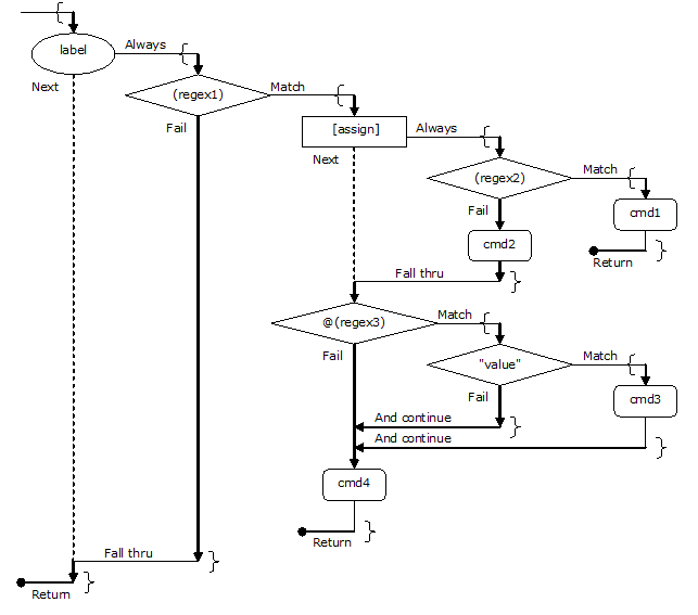
Translators are intended primarily as a way to uniquely identify a line of text and provide a single response. For this reason, the default behavior on a true condition is to execute the subordinate statement and terminate. A simple translator is just a series of patterns to match to the text buffer. The statement following the first matching pattern is executed and the translator stops.
     "value" statement
     "value" statement
     ...
     (regex) statement
     (regex) statement
     ...
However, in some cases you will want to match a line of text to multiple patterns and take the action associated with each. This can be done as follows.
     @"value" statement
     @"value" statement
     ...
     @(regex) statement
     @(regex) statement
     ...
The continue statement, @, performs the subordinate statement and continues to the next statement even if a match was found in the subordinate statement.
The unconditional branch statements, assign and label, have a slightly different default behavior than the conditional branch statements. The unconditional branch statements continue to the next statement by default if a match is not found in the subordinate statement. In the following example, the statement in the third line will execute if the subordinate statement of the assign and label statements, a (regex) statement in both cases, doesn't find a match.
[assign](regex) statement
label(regex) statement
statement
However, like the conditional branch statements, you can use a "continue" statement to ensure they continue to the next statement when a match is found in the subordinate statement.
@[assign](regex) statement
@label(regex) statement
statement
The only other flow control statement is the block statement, which groups a list of statements into a single statement.
(regex) { # if regex is true, execute block and terminate
statement
statement
}
@(regex) { # if regex is true, execute block and continue
statement
statement
}
label{ # execute block and continue if no match
"value" statement
(regex) statement
(regex) statement
}
@label{ # execute block and continue
"value" statement
(regex) statement
(regex) statement
}
The flow of control within a block is the same as it would be outside of a block—the block functions like a subordinate translator.
Translator statements are defined recursively, where statements often contain subordinate statements. A translator script not only has a top to bottom sequence of statements but a statement can have a left to right sequence of elements that form multiple statements within the recursive definition.
Statement: label(regex)[assign]"value":command
Recursion: |-statement-|
|---statement-------|
|---statement----------------|
|---statement------------------------|
|---statement------------------------------|
A subordinate statement refers to a statement within a statement. More specifically, a subordinate statement is the statement to the right of a statement's first element.
You can think of the individual elements that make up a complex statement as cells in a table. Imagine a translator script as a table of complex statements, where each complex statement is a row in the table, and each element of a statement is a cell in a row.
Statement: label(regex)[assign]"value":command
Table: cell cell cell cell cell
Under this model, cells execute left to right, and return True or False values from right to left.
It gets a bit more complicated when you consider that while a statement has only one subordinate statement; a subordinate statement may be a block statement as illustrated here.
label{
(regex) {
[assign] {
"value1" {
: command1
: command2
}
"value2":command3
}
: command4
}
}
You can adapt to this concept by thinking of a translation table, where the elements are cells, as a translation tree, where the elements are nodes.
Statement: label(regex)[ assign]" value1":command1
| | |
| | : command2
| |
| "value2":command3
|
: command4
Tree: node node nodes nodes nodes
Subordinate statements are now branches of the tree. You have elected to represent child nodes as a vertical list, because they execute in a top to bottom order. This means "value1" and "value2" are children of [assign]. The command1 and command2 nodes are children of "value1". When represented this way, each node has a single subordinate branch of the tree and a next sibling link.
Within a branch, you execute nodes in a left to right, top to bottom order. Subordinate branches return a True or False value to their parent node (right to left). When a True value is returned to a node other than @, a True value is returned to the parent. When a False value is returned to an unconditional node, processing continues with the next child node (top to bottom). A @ node always continues to the next child node when the subordinate branch returns. A conditional node returns True on a match, ignoring the return value from the executed subordinate branch. A conditional node continues to the next child node when the match fails. If the end of a child node list is reached, a value of False is returned to the parent node.
You can specify the translation tree above as a table, not using block statements, but may get a little confused about flow of control. Are the last three statements reachable with a common value of (regex)? That topic is addressed in the next section.
Statement: label(regex)[assign]"value1":command1
Statement: label(regex)[assign]"value1":command2
Statement: label(regex)[ assign]" value2":command3
Statement: label(regex):command4
In the previous section, the notion that a translator is a collection of nodes organized as a tree structure was introduced. Furthermore, translator statements are interpreted as "transactions" that update a translation tree.
Here's an example of a valid translator script coded as a table, not using block statements.
(regex1)[assign1]"value1":command1
(regex1)[assign1]"value1":command2
(regex2)[assign2]"value1":command1
Here's the same translator script after it is compiled (loaded by the interpreter) and organized as a tree.
(regex1)[assign1]"value1"{
: command1
: command2
}
(regex2)[assign2]"value1":command1
If the compiler left the script in the original form, you would not get the desired result. In fact, command2 would be unreachable, because whenever (regex1) is true NodeBrain would terminate without executing the second statement.
Instead, the compiler ensures that there is only one branch node with a given specification in the first column of a block. This can cause a "reordering" of statements. Consider the following translator.
"abc":assert abc;
"def":assert def;
"abc":assert cba;
(abc):assert containsAbc;
(def):assert containsDef;
(abc):assert containsCba;
After it is compiled, it looks like this.
"abc"{
:assert abc;
:assert cba;
}
"def":assert def;
(abc) {
:assert containsAbc;
:assert containsCba;
}
(def):assert containsDef;
It is important to understand this reordering. Otherwise, it may not always produce the desired result. For the "value" statements above, it is hard to imagine a different intended result, since the second "abc" would be unreachable if not combined with the first, and the order of the commands associated with "abc" ("assert" commands in this case) is preserved.
However, for the (regex) statements, you can imagine more than one possible expectation of the original ordering. If an input text line contains both (abc) and (def), you may want to execute the assertions in the specified order. If so, you can achieve this with a bit more effort. By putting a label on the first (abc) statement, it no longer merges with the second because it is on a different branch introduced by the label. But the label, by itself, would make the second (abc) unreachable. So you use a "continue" statement on the first (abc) and the (def) statement to make the second (abc) reachable for input containing both (abc) and (def).
@bob(abc):assert containsAbc;
@(def):assert containsDef;
(abc):assert containsCba;
Now you have preserved the original order and ensured that each statement is reachable.
It is appropriate that this be the more difficult intention to implement, because you assume it is the least frequent intention. It is more often the case that you only need to test input text for a given condition once.
Here is an alternate solution for the same intention where you include a second (def) statement.
(abc) {
:assert containsAbc;
(def):assert containsDef;
:assert containsCba;
}
(def):assert containsDef;
This isn't all the potentially unhelpful help the compiler demands to provide. It also assumes that you should match values before regular expression. So the following translator is also reordered.
(a.*c) statement
(de(f|d)) statement
"abc" statement
"zyz" statement
Here's what the compiler decides is better.
"abc" statement
"zyz" statement
(a.*c) statement
(de(f|d)) statement
The compiler's preference is usually better because when there is a large number "value" statement, the translation engine can quickly determine, which, if any, value matches the input by performing a binary search. If there is no value match, then it can continue with the less efficient regular expressions.
Once again you can force the compiler to preserve the original order by using a labeled blocks as shown below. Now the "value" statements are at the top of their block as the compiler insists, and they are executed after the (regex) statements, as you may insist.
@reStmts{
(a.*c) statement
(de(f|d)) statement
}
valueStmts{
"abc" statement
"zyz" statement
}
You may, or may not, want the "continue" on the "reStmts" block. If not, you could simply remove the block.
(a.*c) statement
(de(f|d)) statement
valueStmts{
"abc" statement
"zyz" statement
}
Now the "abc" is unreachable, but that may be intentional, particularly if the value statements are managed as a separate translator. The goal may be to intercept the values matching the regular expressions to prevent the value statements from responding to those cases. Here you have removed to (regex) subordinate statements to suppress response instead of providing an alternate response. Either would be reasonable.
(a.*c)
(de(f|d))
valueStmts~plan/watchedValues/watchedValues.nbx
The important thing is to understand how the compiler reorganizes a translation script so you can direct it to do what you want.
When a translation script (*.nbx file) is loaded, each statement is processed as a transaction applied to the translator tree structure, which is initially empty. By default, each statement is an "insert at bottom" transaction. Each element of a statement is used as a key to select an existing branch node or create a new branch node at the bottom of a block. You could explicitly state that you are adding a node at the bottom of a block by preceding it with a greater than symbol (>).
# Insert at bottom
(abc.*?(\d+))>"abc"
If you want to insert a node at the top of a block, use a less than symbol (<).
# Insert at top
(abc.*?(d\+))<"abc"
The equal symbol (=) is used to replace the contents of a branch or leaf node.
# Update transaction
(abc.*?(d\+))="abc"
"abcdef".27=:assert x=1;
A branch node may be deleted ("pruned") by preceding it with a vertical bar (|). The examples below illustrate the deletion of a value node, regex node, and leaf node (command or file link).
# Delete transactions
(abc.*? (\d+))|"abc"
Fred.(abc.*?(\d+))[$[1]] | (def (\w+))
"abcdef"|5
Note that operations on a leaf node require identification by "line number" within a block. This is because leaf nodes are not uniquely identified by their text since a command may be repeated within a block.
More types of transactions are listed in the next section.
This one page summary is a handy reference. It also seems to validate the claim—the translation language is quite small.
Statements
*- Four concepts sufficient for most translation tasks
"string" - Branch on string match
(regex) 1- Branch on regular expression match
[assign] - Branch unconditionally after projecting new text buffer
label - Branch unconditionally (unconditional branches "fail thru")
{ 2- "Begin" statement block
} - "End" statement block
:command 3- "Command" NodeBrain interpreter---see projection
$file - "Include" statements from file
~file - "Link" to another translator
Projection 4- Compose string from matched text and literal text
[[to here: make subordinate to projection]]
$[-] - Input - full input string ..........
$[~] - Match - String that matches (regex) --(...)---
$[<] - Head - string before $[~] ...(regex) if $[-] before first match
$[>] - Tail - string after $[~] (regex)... is $[-] before first match
$[=] - Assigned text buffer is $[>] before assignment
$[1] - String matching first sub-expression (...(subexpr)...)
$[n] - String matching n'th sub-expression
$[name] - String matching a named sub-expression (?'name'...)
$[_,FR] - Replace character F with character R, where _ is -|~|<|>|=|n
F is " and R is ' by default
$[.?] - One prior to most recent ancestor regex - ? is any of the above
$[..?] - Two prior to most recent ancestor regex
$[...?] - Can continue up from any depth of regex nesting
Control
@branch - "Continue" even if branch returns true
!stmt - Ignore statement - like commenting to end of statement
Transactions
path - branch.branch.branch[.n]
path.stmt - Insert statement reusing existing branches
path?stmt - Show branch after processing statement
^path - Verify path exists
^path+@ - Set "continue" option on branch
^path-@ - Clear "continue" option on branch
^path+! - Set "disabled" option on branch
^path-! - Unset "disabled" option - enable
^path|branch - Prune (delete) branch
^path|n - Prune (delete) leaf statement n (see path)
^path>stmt - Insert at end of branch or after leaf statement n
^path<stmt - Insert at start of branch or after leaf statement n
^path=stmt - Replace branch or leaf statement n within branch
NodeBrain supports multiple forms of symbolic substitution: preprocessor, substitution command, cell definition, cell value, macro, and translator string. Each has a unique syntax as indicated in the right column of boxes in the figure below.
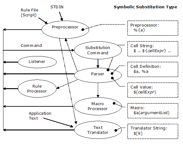
Syntax
|
Preprocessor terms are defined in a separate dictionary from rule terms. They may be assigned values as arguments to nb, as arguments to a rule file, and within a rule file using the %assert directive or the assert command.
nb a=1 b="abc" myscript [global process terms "a" and "b"]
nb myscript,a=2,b=3 [local process terms "a" and "b"]
%assert a="hello"; [directive]
assert %a="hi"; [preprocessor term defined from rule context]
Preprocessor substitution is accomplished by enclosing a term in braces preceded by a percent symbol: "%{term}".
% define x cell "%{a}";
% define %{a} cell 17;
Preprocessor substitution applies to rule files, including standard input (stdin). It is performed on every line of a file before it is processed in any other way, completely independent of command syntax.
This substitution does not apply to commands received by listeners. This is primarily because the notion of conditional interpretation, at least in the form of the multi-line %if directive, doesn't apply well to commands arriving at a listener. However, the global process term dictionary is available to all commands. The ability to update it depends on one's authority, but read access is available to any identity with the ability to issue a command. You will see in the next section how global process terms can be used in symbolic string substitution of a different form.
Syntax
|
String substitution based on cell expressions using terms in the rule dictionary is performed by the substitution command. This step provides a method of composing a command before it is parsed, but an explicit request is required to avoid unnecessary overhead. A symbolic expression of the form ${cellExpression} is replaced by a string representing the value of cellExpression within the active context. For efficiency in handling most commands that do not use symbolic substitution, NodeBrain requires an explicit request for symbolic substitution by starting a command with $ followed by a space.
assert a="abc",b=123.45,c=0.55;
$ assert ${a}=${b},xyz="${b}",n=${b+c};
assert abc=123.45,xyz="123.45",n=124; # command after substitution
We elected not to follow the common practice of using an escape character to delay or prevent substitution (e.g., "\\\$a"). Instead, NodeBrain uses multiple dollar signs ("$${") to delay substitution, giving the programmer control over when substitution occurs.
... ${term} Symbolic substitution is performed on first request
... $${term} Symbolic substitution is performed on second request
... $$${term} Symbolic substitution is performed on third request
Each time symbolic substitution is requested the number of $ symbols is reduced by one.
$ ... $${term} Before substitution
... ${term} After substitiution
$ ... $$${term} Before substitution
... $${term} After substitution
When a substitution request is presented to the interpreter, substitution is performed left to right from the first character to the last character, independent of the statement syntax.
> define x cell "def"
> define y cell "ine z"
> $ ${x}${y} cell "abc"
define z cell "abc" <-- substitution
In context stacks, substitution is performed in the active context. Reduction is followed by symbolic substitution within the new context. When reduction is specified in the action command of a rule, reduction (but not substitution) is preformed in advance (at the time the rule is interpreted).
> define x cell "abc"
> $ define r1 on(a="${x}"):$ - echo x=$${x} was ${x}
define r1 on(a=1):$ - echo x=${x} was abc <-- substitution
> assert a=1,x="xyz";
... rule r1 fires ...
$ - echo x=${x} was abc <-- rule action
: - echo x=xyz was abc <-- substitution
x=xyz was abc
This form of symbolic substitution, while normally used with rule dictionary terms, can also be used with terms in the process dictionary. This is because a global process term is accessible from any rule context in the form %term.
%{term} - Process string substitution only for rule files.
${%term} - Cell string substitution available anywhere.
To avoid getting a local process term, your can explicitly specify back up to the global context.
${%..term} - Bypass local terms if any.
Syntax
|
When an identifier in a formula is preceded by a dollar sign ($), it is called a symbolic cell name and is interpreted as if the identifier's current formula had been specified. You illustrate this with a sequence of three assertions, first without a $ and then with it.
# without "$"
assert a=2,b=3,x==a*b;
assert y==x+21;
assert x==a+b; # this assertion changes y
# with "$"
assert a=2,b=3,x==a*b;
assert y==$x+21; # same as y==(a*b)+21
assert x==a+b; # no change to y
Use of symbolic cell names only impacts assertions using == since = resolves the current value of the formula anyway.
assert a=2,b=3,x==a*b;
# The next three statements produce the same result: y=27
assert y=$x+21;
assert y=x+21;
assert y=27;
Statement parsing and execution are two distinct phases. Cell names are replaced by the parser using their current definition. This is illustrated by the following example. The definition of x is not changed to (a*b) until the statement is executed, so $x is replaced by the parser with the current definition of x at parse time: (a+b).
assert x==a+b;
assert x==a*b,y==$x+21; # y==(a+b)+21
In the previous example, execution directly follows parsing, but this is not the case with rules. In the following example, x may take on many definitions between the time the rule is parsed and the time the rule fires and performs the assertion. Because substitution occurs at parse time, changes to x after the rule is parsed have no impact on the assertion performed when the rule fires.
assert x==a+b;
define r1 on(a>5 and b<20) x==a*b,y==$x+21; # y==(a+b)+21
assert x==a/b;
...
Command actions (e.g., on(condition):command) are parsed when the rule fires.
Syntax
|
When a symbolic cell expression "$(cellExpression)" is specified within a cell expression, it is replaced by the current value of the symbolic cell expression.
assert a=2,b=3,?c;
assert y==$(a*b)+c; # same as y==6+c;
Like symbolic cell names, a symbolic cell expression is only useful when defining a term using the == operator, since = resolves the current value of the cell expression anyway.
Syntax: Macro Definition
|
Syntax: Macro Command
|
A macro is defined to provide a model for macro command expansion. A macro command accepts positional arguments or keyword arguments. In the following example, m1 is defined to have two positional parameters (a and b) and one keyword parameter (c);
define m1 macro(a,b:c=5):assert x=%%{a}*%%{b}/%%{c};
When you use a macro, you must specify the expected number of positional arguments, but the keyword arguments are optional.
> $m1(2,7);
$ assert x=2*7/5;
> $m1(3,5:c=12);
$ assert x=3*5/12;
Macros may be used as a typing shortcut, a way of making code easier to read, or to provide a common point of maintenance. Consider the following macro for alerting an alarm node.
> define myalert macro(text:severity="normal",group="OS")\
alarm. alert severity="%%{severity}", \
group="%%{group}",text="%%{text}";
Here we show the use of this macro and the expansion.
> $myalert("Hello");
$ alarm. alert severity="normal",group="OS",text="Hello";
This appendix shows how special symbols are used in the context of various constructs of the language. An alpha character string is indicated with "a", a string of numeric digits with "9", and a cell expression with "e". We reference the following contexts as constructs within the language.
| Source | - Anywhere in a source file or macro string
|
| Command | - Anywhere in a command line
|
| Substitution | - Within a symbolic substitution expression ${...}
|
| Verb | - First non-blank characters of a command following context prefix.
|
| Type | - Where a type is expected in a define or declare statement.
|
| Identifier | - Where an identifier is expected.
|
| Cell | - Cell expression, when not in one of the following contexts.
|
| Sequence | - Within a sequence {...}
|
| TimeSeq | - Within a time sequence ~{...} or ~(...{...}... )
|
| TimeExpr | - Within a time expression ~(...).
|
We are still considering the ideas in boldface—they have not been implemented.
| Symbol | Context | Description
|
|---|---|---|
| %{9...} | source | Positional parameter symbolic substitution
|
| %{a...} | source | Local term symbolic substitution
|
| %a | source | Source Directive (column 1)
|
| ${...} | command | Symbolic substitution directive
|
| {...} | substitution | Nested symbolic substitution directive
|
| # | verb | Comment
|
| $ ... | verb | Symbolic substitution directive
|
| $a(...) | verb | Macro expansion directive
|
| a. | verb | Context prefix
|
| ^ | verb | Direct message to stdout
|
| - | verb | Execute a host command
|
| = | verb | Spawn a process to run a host command
|
| =[a] | verb | Spawn a process switching users
|
| a: ... | verb | Direct a command to a node
|
| ` | verb | Abbreviation for assert (backtick)
|
| { | verb | Sequence {...}—starts a thread
|
| %a | identifier | Local term
|
| a.a | identifier | Glossary selection—separates levels of qualification
|
| .a | identifier | Term in active context glossary
|
| ..a | identifier | Term in parent context glossary
|
| _.a | identifier | Term in root context glossary
|
| '...' | identifier | Term containing special symbols
|
| _a | identifier | Special terms created by nodes
|
| %_a | identifier | Special built-in local terms (e.g., %_hostname)
|
| Symbol | Context | Description
|
|---|---|---|
| "..." | cell | String |
| (...) | cell | Subordinate cell expression
|
| $a | cell | Symbolic reference to the definition of a
|
| $(e) | cell | Cell expression evaluated at parse time
|
| & | cell | Boolean operator—AND
|
| | | cell | Boolean operator—OR
|
| ! | cell | Boolean operator—NOT
|
| ^ | cell | Flip-flop operator
|
| ~(...) | cell | Time condition
|
| ~{...} | cell | Time sequence
|
| ~^(...) | cell | Time Delay Condition—delay transition to True
|
| ~^!(...) | cell | Time Delay Condition—delay transition to False
|
| ~^?(...) | cell | Time Delay Condition—delay transition to Unknown
|
| {...} | cell | Sequence
|
| ; | Sequence | Statement terminator
|
| * | Sequence | Repeat indefinitely
|
| =e; | Sequence | Set value to cell expression
|
| `...; | Sequence | Assertion (backtick)
|
| : ...; | Sequence | Command
|
| / | Sequence | Set value to True
|
| \ | Sequence | Set value to False
|
| {...} | Sequence | Sequence block
|
| (...) | Sequence | Time condition
|
| } | Sequence | Sequence terminator
|
| + | TimeSeq | Sign for time unit multiplier
|
| - | TimeSeq | Sign for time unit multiplier
|
| / | TimeSeq | Set value to True
|
| \ | TimeSeq | Set value to False
|
| ({...) | TimeSeq | Time condition
|
| {...} | TimeSeq | Sequence block
|
| } | TimeSeq | Sequence terminator
|
| Symbol | Context | Description
|
|---|---|---|
| =a | TimeExpr | Prefix Operators
|
| | |
| |
| # |
| |
| ! |
| |
| & |
| |
| ~ |
| |
| % |
| |
| , | Infix Operators
| |
| . |
| |
| ! |
| |
| # |
| |
| & |
| |
| | |
| |
| % |
| |
| [...] | TimeExpr | Index List (indexed selection)
|
| , | TimeExpr Index List | Index union and range separators
|
| _ |
| |
| .. |
| |
| (...) | TimeExpr | Sub-expression
|
| a (...) | TimeExpr | Sub-expression
|
| , | TimeExpr Parameter List | Parameter union and range separators
|
| _ |
| |
| .. |
| |
| / | TimeExpr Parameter | Parent parameter separators: day(12/25) hour(12@10) minute(12:10)
|
| @ |
| |
| : |
|
In many situations, an awareness of transitional features helps to explain the interpreter's response to an otherwise undocumented syntax. These features fall into three categories: (1) experimental, (2) deprecated, and (3) obsolete. The first two categories are supported by the interpreter, but you should avoid them. Avoid experimental features (except for experimentation) because the design is unstable and perhaps not fully implemented. Avoid deprecated features because they have been replaced and will eventually be obsolete. Obsolete features are not supported by the documented release, but were supported by an earlier release.
An expression evaluation shortcut makes it easy to test expressions.
?(expression)
A command option prefix allows options to be set for processing individual commands.
(trace,...) command
Logging options are supported at the node (context) level. If you don't need or want an audit log of every rule that fires, you can turn off the audit trail.
context. use(hush)
context. use(!hush)
context. use(audit)
context. use(!audit)
context. use(trace)
context. use(!trace)
A global "audit" option sets a default option for all nodes. There are eight silly ways to set one option on or off.
nb -a [audit]
nb -A [noAudit]
nb --audit
nb --noAudit
set a
set A
set audit
set noAudit
The default is "audit" (on). There is no harm in leaving audit on unless you decide it is just spitting out too much information. Once your rules have been tested, you can switch to the -A option.
#!/usr/local/bin/nb -A
...
Use of a deprecated syntax will still work but will generate a warning message. You should update your rule files to the current syntax to avoid problems later when the old syntax becomes obsolete.
Avoid the use of "expert" when defining a node.
Deprecated:
> define term expert ...;
Current:
> define term node ...;
Avoid the use of a double question mark (??) for the Unknown value. Use a single question mark (?) instead.
Avoid the use of a double tilde (~~) for regular expression matching. Use a single tilde (~) instead.
If you have NodeBrain rules that use obsolete features, the current interpreter will normally generate error messages. It is possible, particularly if you upgraded NodeBrain skipping multiple releases without upgrading your rules, that an old syntax has been reintroduced with a new interpretation.
Avoid defining listeners. Instead, define nodes using the associated skill. Skills are documented in the NodeBrain Module Reference.
Obsolete:
> define term listener type="type",...;
Current:
> define term node skill (...);
| Listener Type | Node Skill
|
|---|---|
| FIFO | pipe.reader
|
| LOG | audit
|
| NBP | peer.reader
|
| NBQ | peer
|
| SMTP | smtp.reader
|
Avoid declaring brains. Instead, define a peer node.
Obsolete:
> declare term brain...;
Current:
> define term node peer(...);
Avoid using remote command prefixes. Instead use peer node commands.
Obsolete:
> >brain command
> \brain command
> /brain command
Current:
> node: command
Avoid the portray command. The peer skill portrays the identity specified in the node declaration.
Obsolete:
> portray identity;
Current:
> define term node peer("identity@...");
Use the -: or =: commands instead of the consult command.
Obsolete:
> consult consultantScript
Current:
> -: servantScript
The address command is no longer supported to address subsequent interactive commands to a specific local or remote context. See the single quote special symbol command for similar functionality.
The define statement no longer recognizes the previously deprecated types of context, condition, or string. The context type is replaced by node, although the deprecated expert is still supported. The condition and string types are replaced by cell.
The following commands are obsolete.
default- see%defaultdirectivelet- see%assertdirective
The + prefix is obsolete for node commands.
Obsolete:
> +node(argList):command
Current:
> node(argList):command
Nested substitution expressions require reduction directives. The old syntax was abandoned because it was seldom used and incompatible with the transition to supporting cell expressions for symbolic substitution instead of just simple terms.
Obsolete:
> ... ${{term1}{term2}}
Current:
> $ ... $${${term1}${term2}}
The system and exec commands are no longer supported. See - and = special symbol commands. These are collectively called the "servant" command.
Obsolete:
> (system|exec) shellCommand
Current:
> (-|=)shellCommand
A context prefix may no longer be terminated by a space. In earlier releases a defined context (node name) was recognized in the place of a verb. It will now be interpreted as a verb unless terminated by the folliwng symbols:
. , ( :
Obsolete:
> context verb body
> fred define r1 on(a=1 and b=2);
Current:
> verb body
> define rer1 on(a=1 and b=2);
> context. verb body
> fred. define r1 on(a=1 and b=2);
> context [(args)]:command
> fred(1);
> fred:command
> fred(1):command
NodeBrain is free software; you can modify and/or redistribute it, including this document, under the terms of either the MIT License (Expat) or the NodeBrain License.
MIT License
Copyright © 2014 Ed Trettevik <eat@nodebrain.org>
Permission is hereby granted, free of charge, to any person obtaining a copy of this software and associated documentation files (the "Software"), to deal in the Software without restriction, including without limitation the rights to use, copy, modify, merge, publish, distribute, sublicense, and/or sell copies of the Software, and to permit persons to whom the Software is furnished to do so, subject to the following conditions:
The above copyright notice and this permission notice shall be included in all copies or substantial portions of the Software.
THE SOFTWARE IS PROVIDED "AS IS", WITHOUT WARRANTY OF ANY KIND, EXPRESS OR IMPLIED, INCLUDING BUT NOT LIMITED TO THE WARRANTIES OF MERCHANTABILITY, FITNESS FOR A PARTICULAR PURPOSE AND NONINFRINGEMENT. IN NO EVENT SHALL THE AUTHORS OR COPYRIGHT HOLDERS BE LIABLE FOR ANY CLAIM, DAMAGES OR OTHER LIABILITY, WHETHER IN AN ACTION OF CONTRACT, TORT OR OTHERWISE, ARISING FROM, OUT OF OR IN CONNECTION WITH THE SOFTWARE OR THE USE OR OTHER DEALINGS IN THE SOFTWARE.
NodeBrain License
Copyright © 2014 Ed Trettevik <eat@nodebrain.org>
Permission to use and redistribute with or without fee, in source and binary forms, with or without modification, is granted free of charge to any person obtaining a copy of this software and included documentation, provided that the above copyright notice, this permission notice, and the following disclaimer are retained with source files and reproduced in documention included with source and binary distributions.
Unless required by applicable law or agreed to in writing, this software is distributed on an "AS IS" BASIS, WITHOUT WARRANTIES OR CONDITIONS OF ANY KIND, either express or implied.